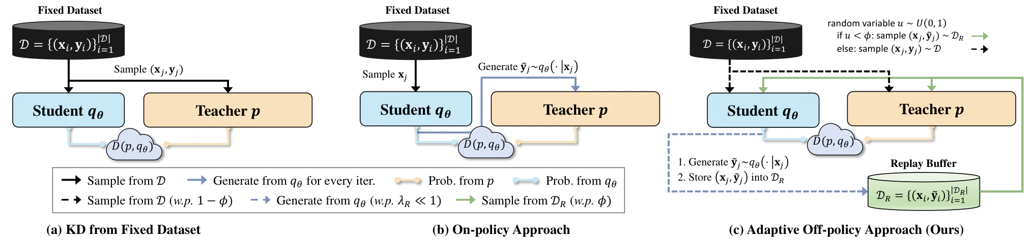
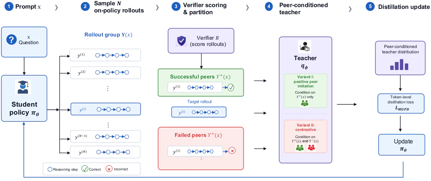
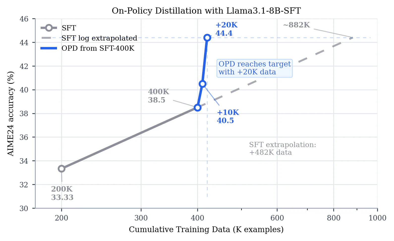
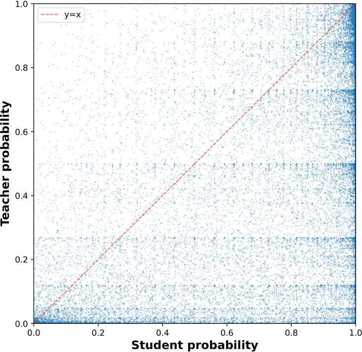
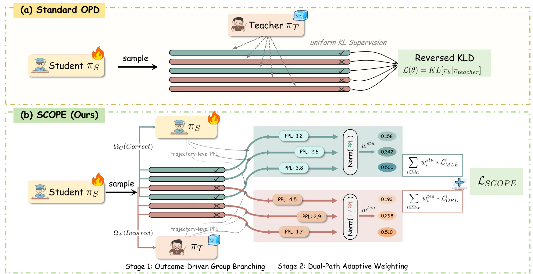
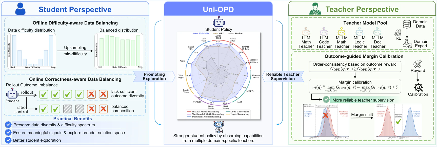
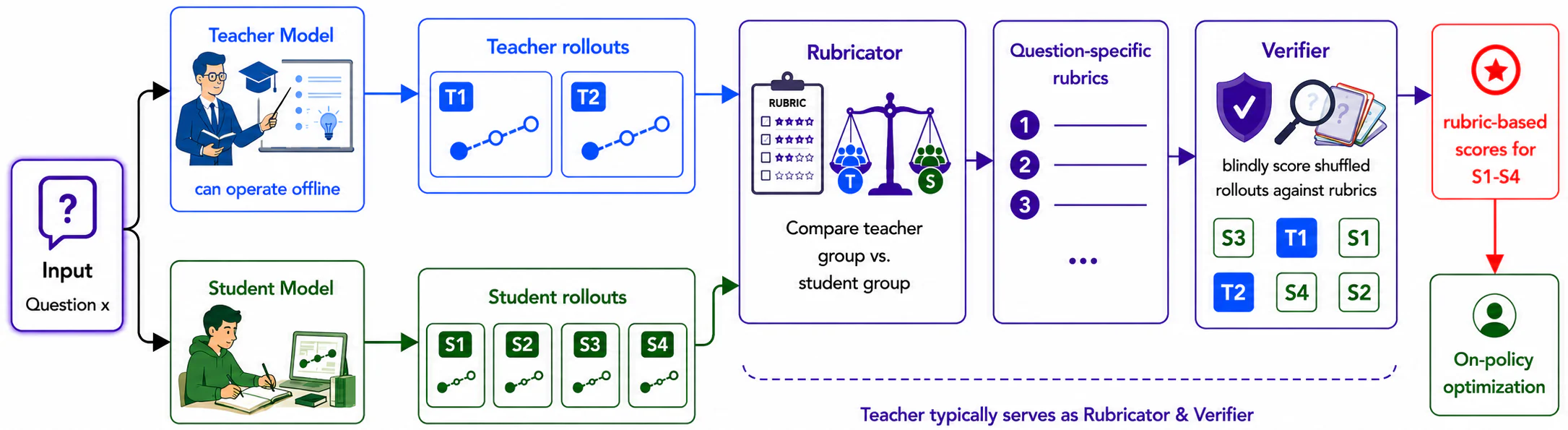
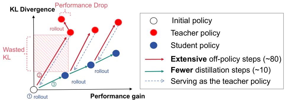
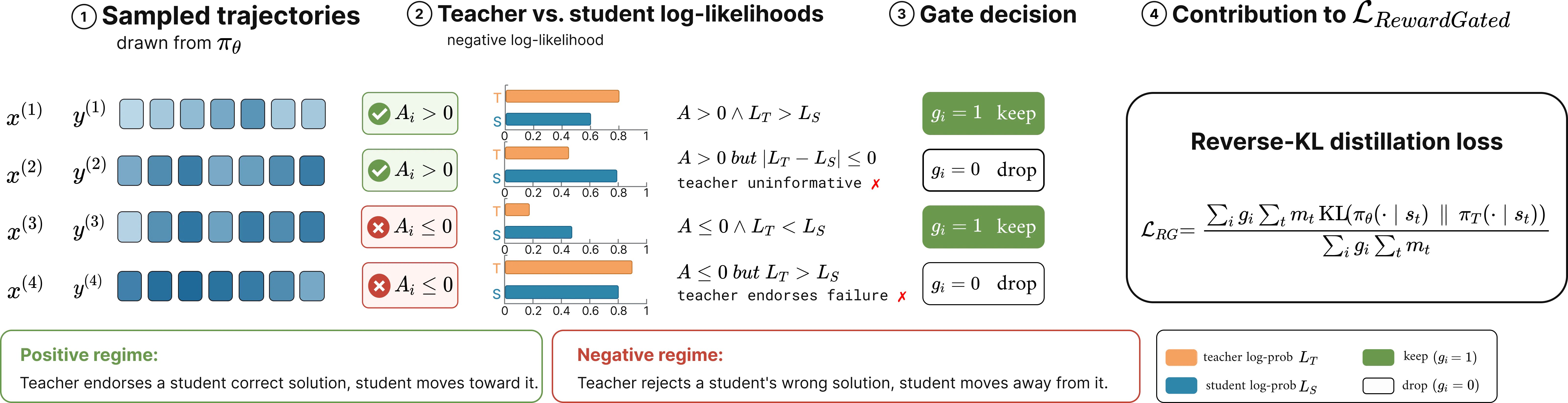
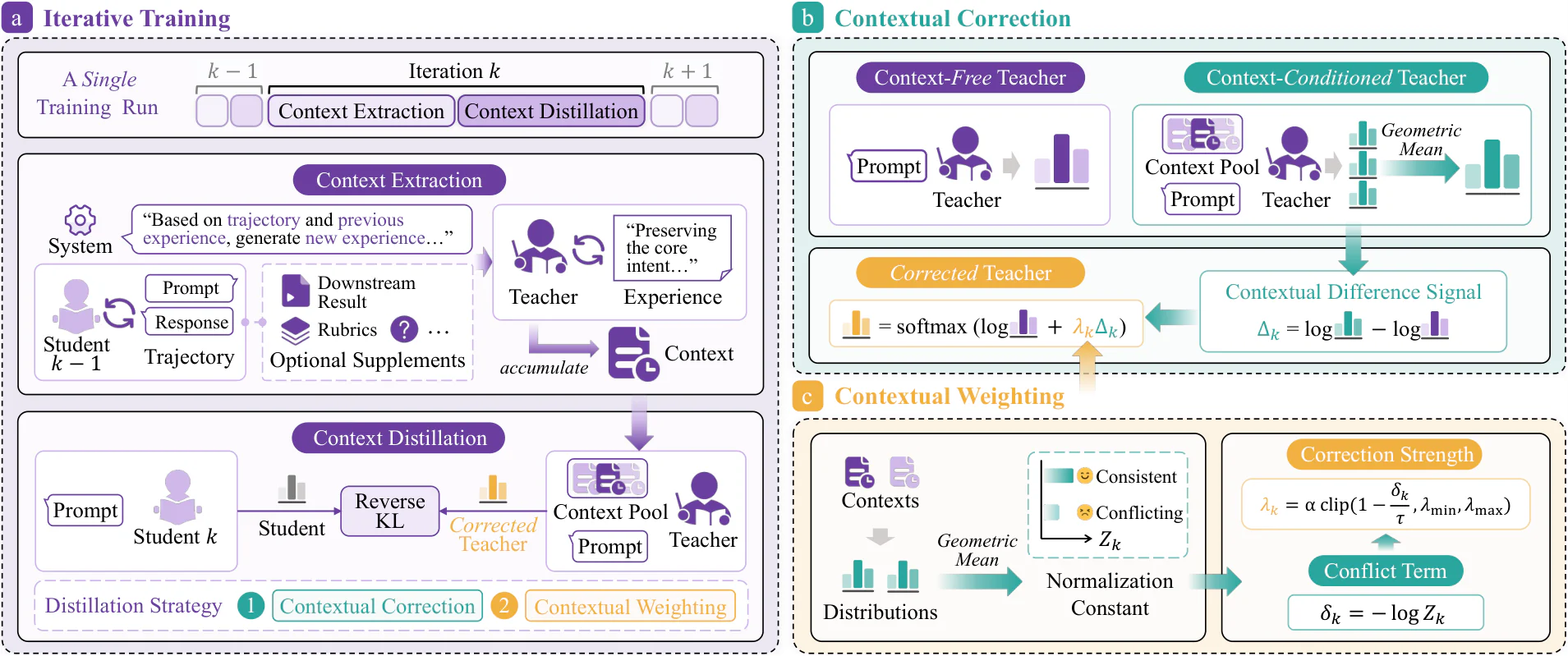
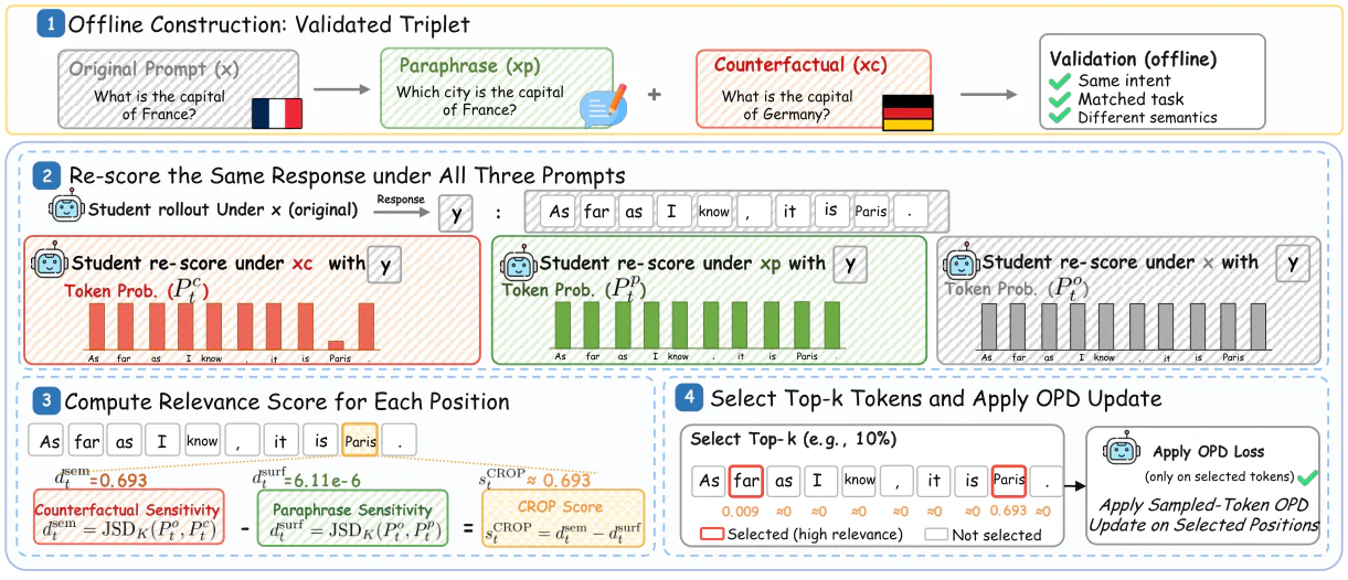
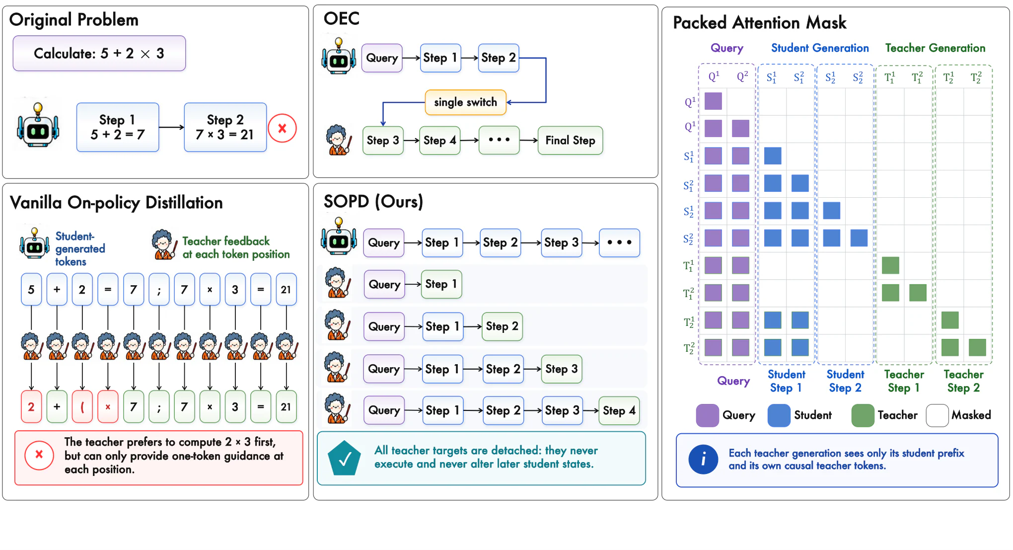
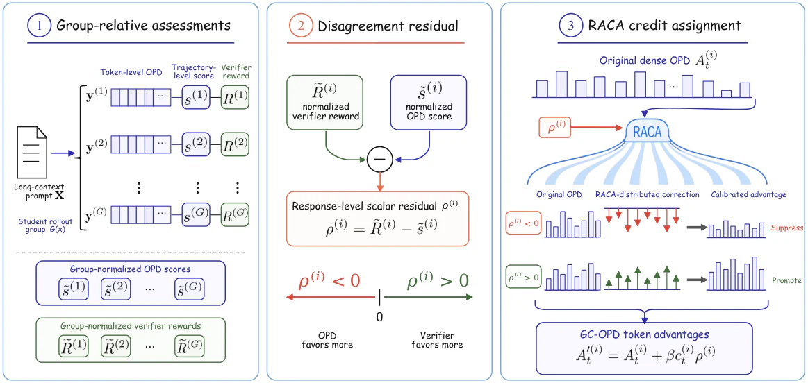
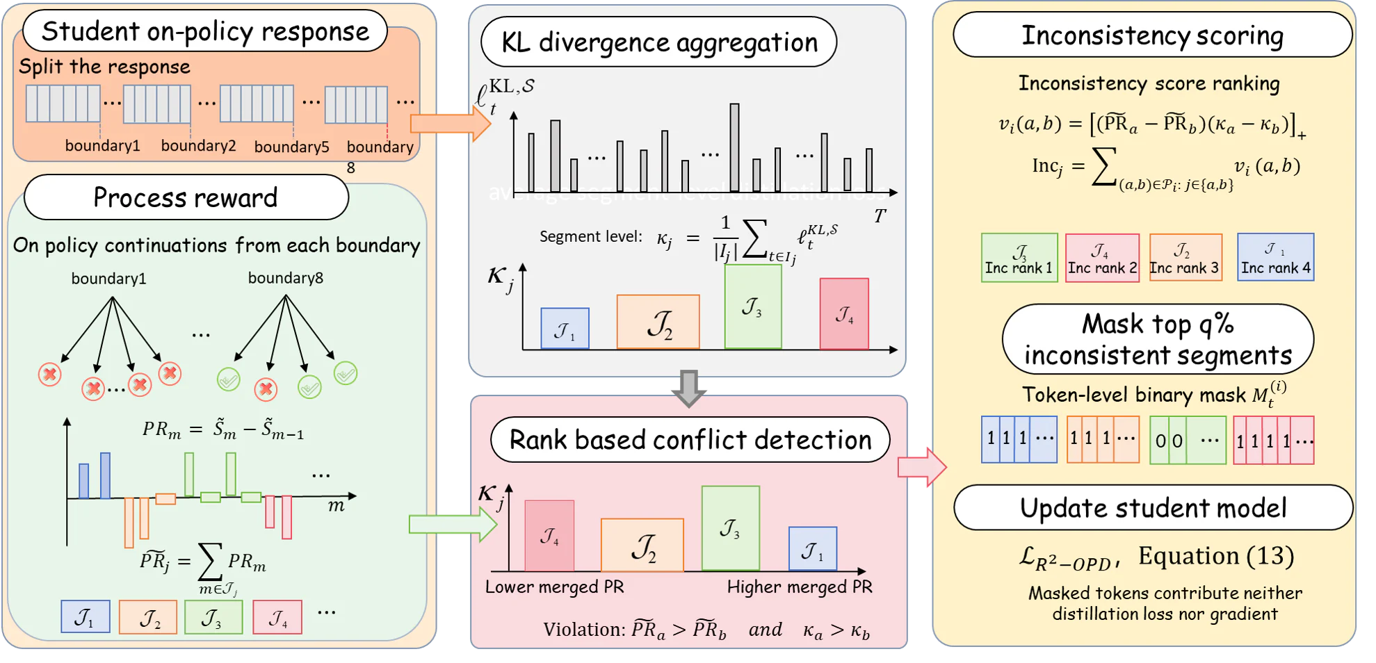
Figure 4: KD from fixed dataset, on-policy approach, and DistiLLM adaptive off-policy approach with replay buffer and decreasing replay ratio. Source: arXiv 2402.03898v2; CC BY 4.0.Figure 4: KD from fixed dataset, on-policy approach, and DistiLLM adaptive off-policy approach with replay buffer and decreasing replay ratio. Source: arXiv 2402.03898v2; CC BY 4.0.
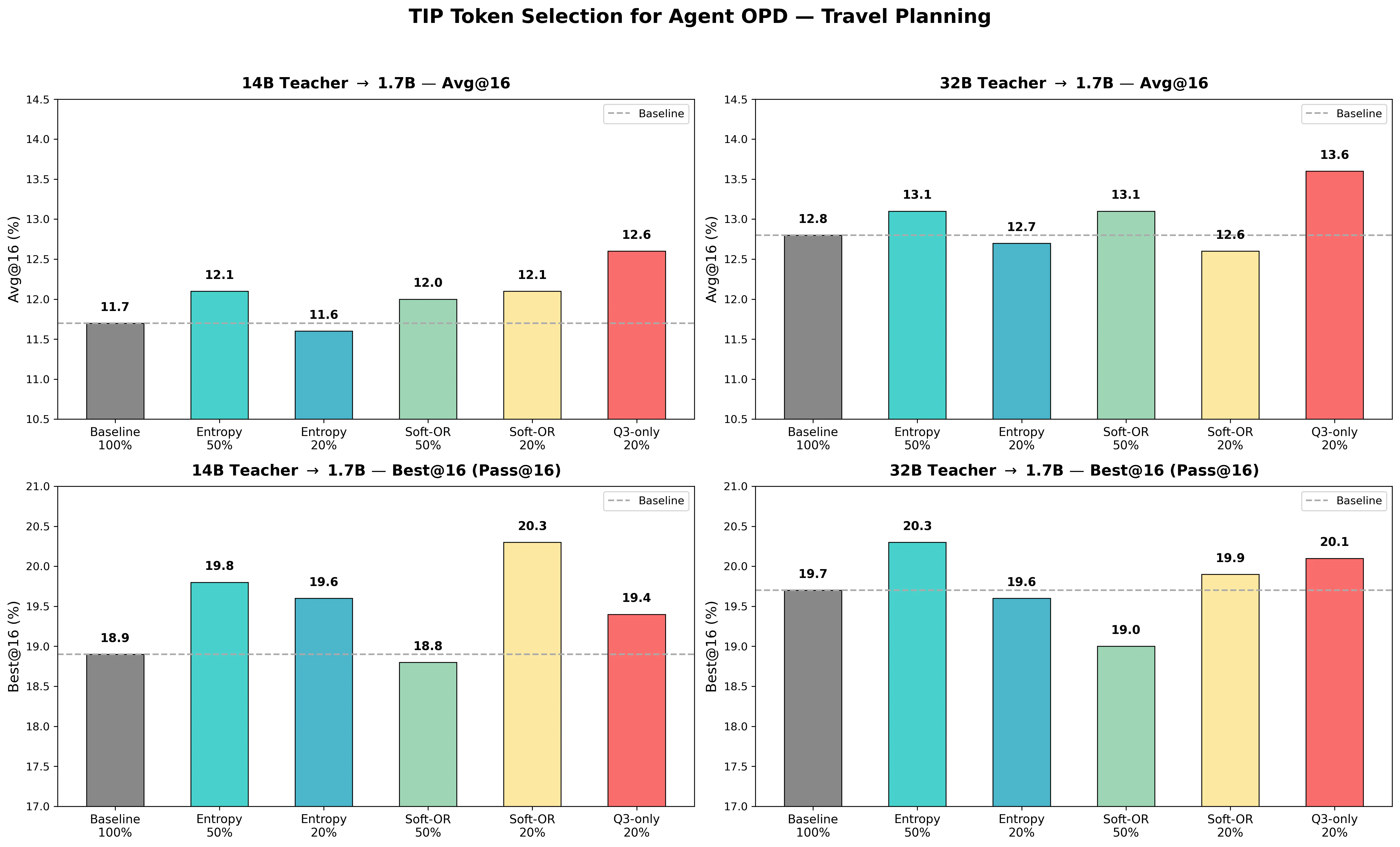
Figure 4 : Token selection for agentic OPD on 20% held-out travel-planning queries. Top row : Avg@16; Bottom row : Best@16 (Pass@16). Within each row the left panel uses the 14B teacher and the right panel uses the 32B teacher. Q3-only 20% matches or exceeds the full-token baseline in every setting, consistent with Table 7 . Best@16 results show the same pattern: overconfident-token training improves the upper tail of performance, not just the mean. Source: https://arxiv.org/html/2604.14084v4/data_figures/planner_agentic.png; license: unknown.Figure 4 : Token selection for agentic OPD on 20% held-out travel-planning queries. Top row : Avg@16; Bottom row : Best@16 (Pass@16). Within each row the left panel uses the 14B teacher and the right panel uses the 32B teacher. Q3-only 20% matches or exceeds the full-token baseline in every setting, consistent with Table 7 . Best@16 results show the same pattern: overconfident-token training improves the upper tail of performance, not just the mean. Source: https://arxiv.org/html/2604.14084v4/data_figures/planner_agentic.png; license: unknown.
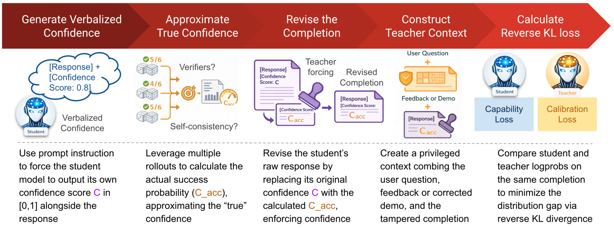
Figure 5: Overview of the CaOPD Framework. The pipeline consists of five stages: (1) querying the student for a base response with verbalized confidence, (2) approximating the true empirical confidence via student rollouts and an objective verifier, (3) revising the completion by replacing the original confidence tokens with the empirical success rate, (4) constructing the privileged teacher context with the same revised confidence, and (5) computing the per-token reverse KL between the student and teacher distributions on the revised completion. Source: https://arxiv.org/html/2604.16830v1/caopd_method.png; license: unknown.Figure 5: Overview of the CaOPD Framework. The pipeline consists of five stages: (1) querying the student for a base response with verbalized confidence, (2) approximating the true empirical confidence via student rollouts and an objective verifier, (3) revising the completion by replacing the original confidence tokens with the empirical success rate, (4) constructing the privileged teacher context with the same revised confidence, and (5) computing the per-token reverse KL between the student and teacher distributions on the revised completion. Source: https://arxiv.org/html/2604.16830v1/caopd_method.png; license: unknown.
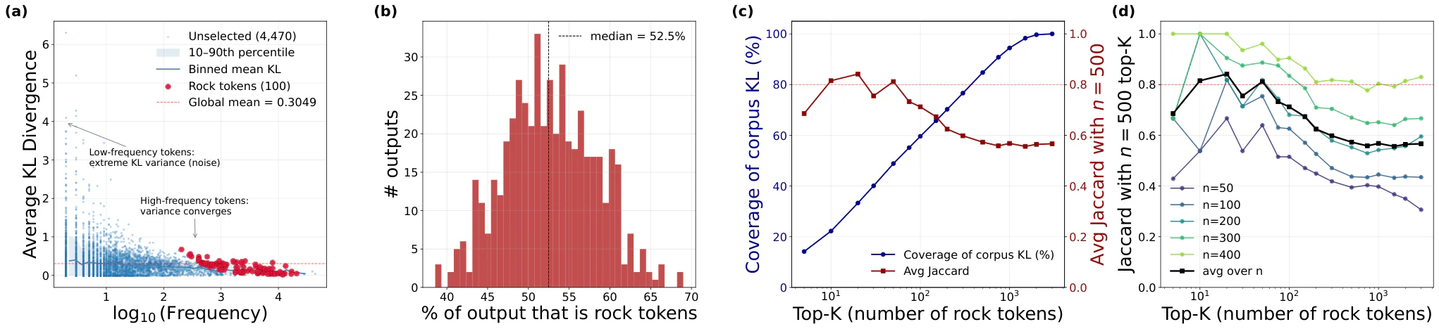
Figure 2: Empirical identification and stability of Rock Tokens. (a) Per-token KL ℓ ^ v \widehat{\ell}_{v} vs. frequency on N = 500 N{=}500 MATH-500 trajectories: rare tokens are noise-dominated, while the Rock Score R ( v ) R(v) isolates true Rock Tokens (red) at the upper edge of stable frequency bands. (b) Per-sequence Rock-Token density (median 18.5 % 18.5\% ). (c) Cumulative loss coverage (blue) and selection stability (red) vs. cutoff K K ; K = 100 K{=}100 balances reproducibility with ≈ 60 % \approx 60\% coverage of the distillation burden. (d) Jaccard ranking robustness across sample sizes n ∈ [ 50,400 ] n\in[50,400] : the top- 100 100 selection is stable, larger cutoffs degrade. Source: https://arxiv.org/html/2605.09253v4/paper_figure1_combined.png; license: unknown.Figure 2: Empirical identification and stability of Rock Tokens. (a) Per-token KL ℓ ^ v \widehat{\ell}_{v} vs. frequency on N = 500 N{=}500 MATH-500 trajectories: rare tokens are noise-dominated, while the Rock Score R ( v ) R(v) isolates true Rock Tokens (red) at the upper edge of stable frequency bands. (b) Per-sequence Rock-Token density (median 18.5 % 18.5\% ). (c) Cumulative loss coverage (blue) and selection stability (red) vs. cutoff K K ; K = 100 K{=}100 balances reproducibility with ≈ 60 % \approx 60\% coverage of the distillation burden. (d) Jaccard ranking robustness across sample sizes n ∈ [ 50,400 ] n\in[50,400] : the top- 100 100 selection is stable, larger cutoffs degrade. Source: https://arxiv.org/html/2605.09253v4/paper_figure1_combined.png; license: unknown.
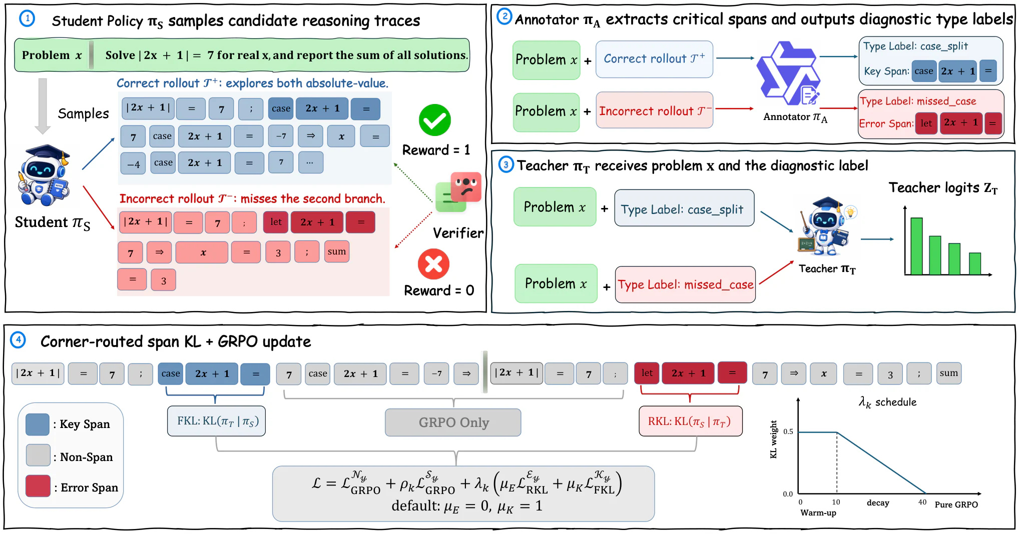
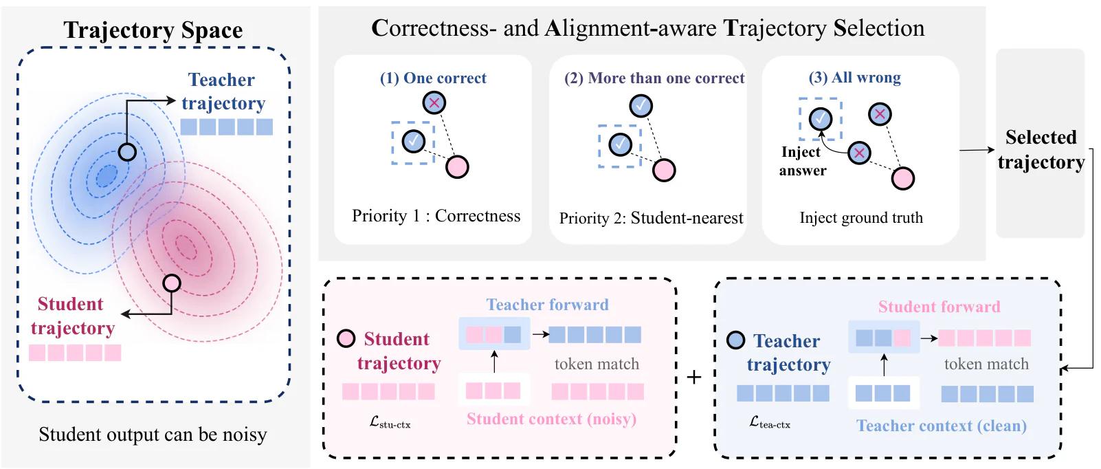
Figure 2 : TRACE pipeline: (1) student samples rollout y ^ \hat{y} and verifier returns R R ; (2) annotator π A \pi_{A} produces both a span mask and a coarse type label; (3) teacher receives the type label as a private diagnostic prefix and computes logits causally on y ^ < t \hat{y}_{<t} ; (4) routed KL action on each span class — the default is FKL on 𝒦 y \mathcal{K}_{y} with no-KL on ℰ y \mathcal{E}_{y} and 𝒩 y \mathcal{N}_{y} — combined with GRPO on 𝒩 y \mathcal{N}_{y} and the KL weight decaying to zero after warm-up. Source: https://arxiv.org/html/2605.10194v1/trace_final.png; license: unknown.Figure 2 : TRACE pipeline: (1) student samples rollout y ^ \hat{y} and verifier returns R R ; (2) annotator π A \pi_{A} produces both a span mask and a coarse type label; (3) teacher receives the type label as a private diagnostic prefix and computes logits causally on y ^ < t \hat{y}_{<t} ; (4) routed KL action on each span class — the default is FKL on 𝒦 y \mathcal{K}_{y} with no-KL on ℰ y \mathcal{E}_{y} and 𝒩 y \mathcal{N}_{y} — combined with GRPO on 𝒩 y \mathcal{N}_{y} and the KL weight decaying to zero after warm-up. Source: https://arxiv.org/html/2605.10194v1/trace_final.png; license: unknown.
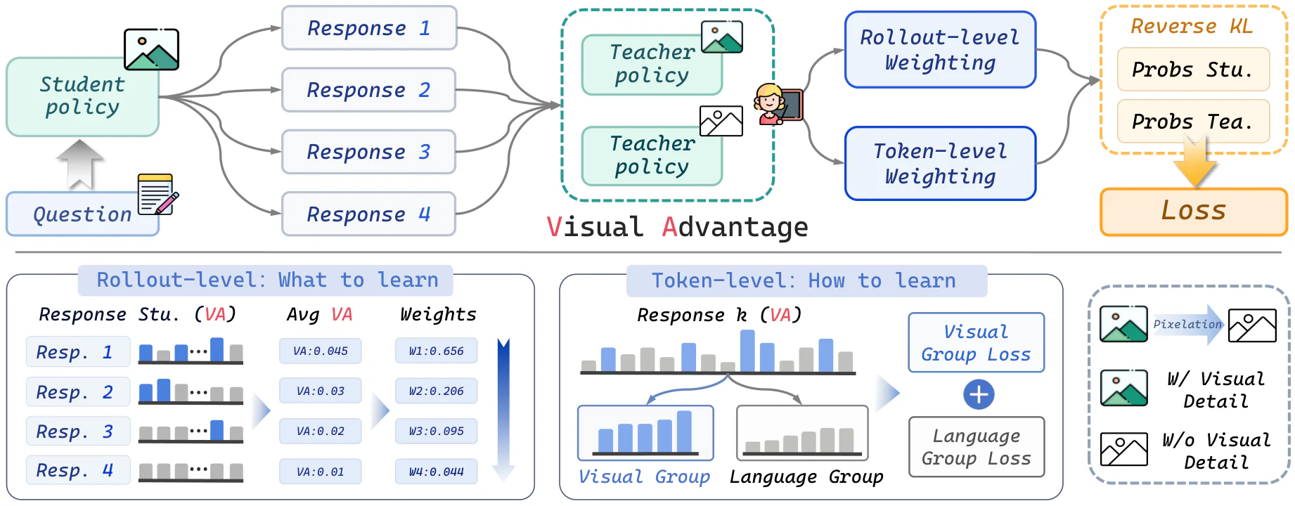
Figure 3 : Overview of Visual-Advantage On-Policy Distillation (VA-OPD). The teacher scores each token with and without fine-grained visual detail; the log-prob difference gives the per-token visual advantage (VA). VA drives reverse-KL distillation at two granularities: rollout-level reweighting by relative VA ( what to learn ) and token-level KL split into high- and low-VA groups ( how to learn ). Source: https://arxiv.org/html/2605.21924v1/method.png; license: unknown.Figure 3 : Overview of Visual-Advantage On-Policy Distillation (VA-OPD). The teacher scores each token with and without fine-grained visual detail; the log-prob difference gives the per-token visual advantage (VA). VA drives reverse-KL distillation at two granularities: rollout-level reweighting by relative VA ( what to learn ) and token-level KL split into high- and low-VA groups ( how to learn ). Source: https://arxiv.org/html/2605.21924v1/method.png; license: unknown.
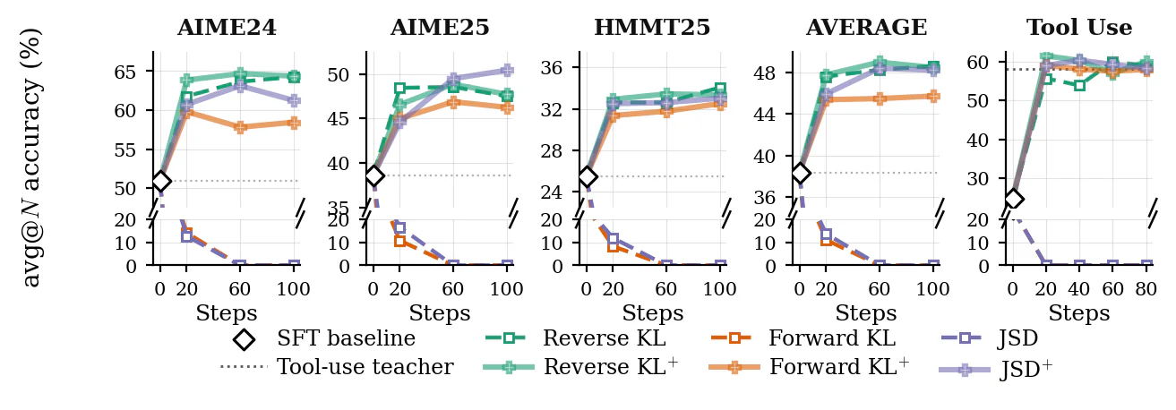
Figure 1: Training dynamics of OPD vs. OPD+ across different steps: we report average accuracy avg@32 ( ↑ \uparrow ) on three math benchmarks (AIME 24, AIME 25, HMMT 25), their average, and an agentic Tool Use task (rightmost panel). Solid lines with markers ( + + ) represent our corrected OPD+ variants ( w ( u ) w(u) ), while dashed lines ( □ \square ) denote standard OPD baselines ( − f ( u ) -f(u) ). OPD+ consistently accelerates early convergence or prevents catastrophic training collapse. Source: https://arxiv.org/html/2606.01039v1/Figures/opd.png; license: unknown.Figure 1: Training dynamics of OPD vs. OPD+ across different steps: we report average accuracy avg@32 ( ↑ \uparrow ) on three math benchmarks (AIME 24, AIME 25, HMMT 25), their average, and an agentic Tool Use task (rightmost panel). Solid lines with markers ( + + ) represent our corrected OPD+ variants ( w ( u ) w(u) ), while dashed lines ( □ \square ) denote standard OPD baselines ( − f ( u ) -f(u) ). OPD+ consistently accelerates early convergence or prevents catastrophic training collapse. Source: https://arxiv.org/html/2606.01039v1/Figures/opd.png; license: unknown.
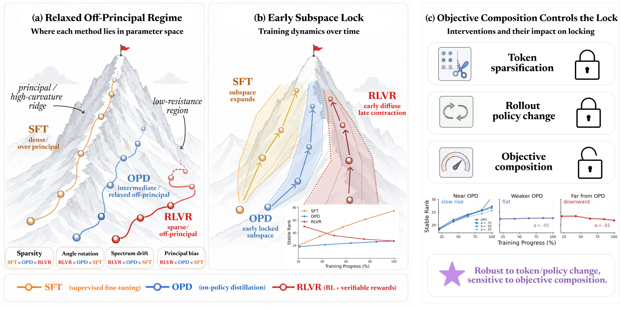
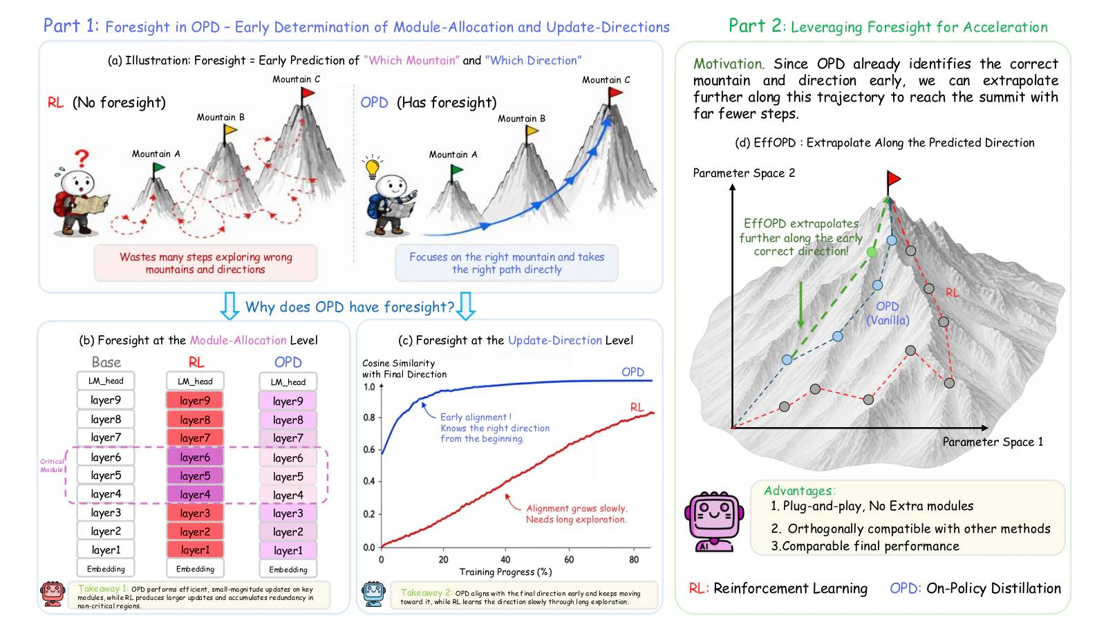
Figure 1: Optimization geometry of OPD compared with SFT and RLVR. (a) OPD occupies a relaxed off-principal regime between dense principal-aligned SFT updates and sparse off-principal RLVR updates. (b) OPD rapidly enters a locked low-dimensional subspace during training. (c) The lock is robust to token and rollout perturbations, but sensitive to objective composition. Source: https://arxiv.org/html/2606.07082v3/Main.png; license: unknown.Figure 1: Optimization geometry of OPD compared with SFT and RLVR. (a) OPD occupies a relaxed off-principal regime between dense principal-aligned SFT updates and sparse off-principal RLVR updates. (b) OPD rapidly enters a locked low-dimensional subspace during training. (c) The lock is robust to token and rollout perturbations, but sensitive to objective composition. Source: https://arxiv.org/html/2606.07082v3/Main.png; license: unknown.
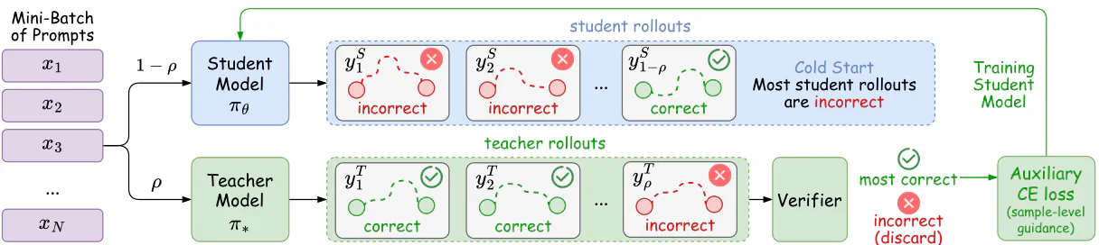
Figure 2: Sample-level Phased Teacher Sampling (PTS). A mini-batch is split into student on-policy rollouts and a small fraction of teacher rollouts. Verified teacher trajectories are retained and used as an auxiliary CE anchor, while incorrect teacher trajectories are discarded. The teacher-guidance weight is annealed from warm-up to zero, so the asymptotic training distribution remains on-policy. Source: https://arxiv.org/html/2606.09304v1/SG-OPD-PTS.png; license: unknown.Figure 2: Sample-level Phased Teacher Sampling (PTS). A mini-batch is split into student on-policy rollouts and a small fraction of teacher rollouts. Verified teacher trajectories are retained and used as an auxiliary CE anchor, while incorrect teacher trajectories are discarded. The teacher-guidance weight is annealed from warm-up to zero, so the asymptotic training distribution remains on-policy. Source: https://arxiv.org/html/2606.09304v1/SG-OPD-PTS.png; license: unknown.
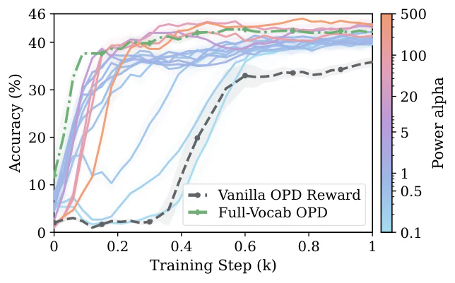
Figure 4: Training dynamics across α \alpha for a Qwen3-0.6B-Base student: (a,b) accuracy and length with a Qwen3-4B teacher; (c,d) accuracy and length with a Qwen3-8B teacher. Source: https://arxiv.org/html/2606.17199v1/fig4a_alpha_acc_s0p6b_t4b.png; license: unknown.Figure 4: Training dynamics across α \alpha for a Qwen3-0.6B-Base student: (a,b) accuracy and length with a Qwen3-4B teacher; (c,d) accuracy and length with a Qwen3-8B teacher. Source: https://arxiv.org/html/2606.17199v1/fig4a_alpha_acc_s0p6b_t4b.png; license: unknown.
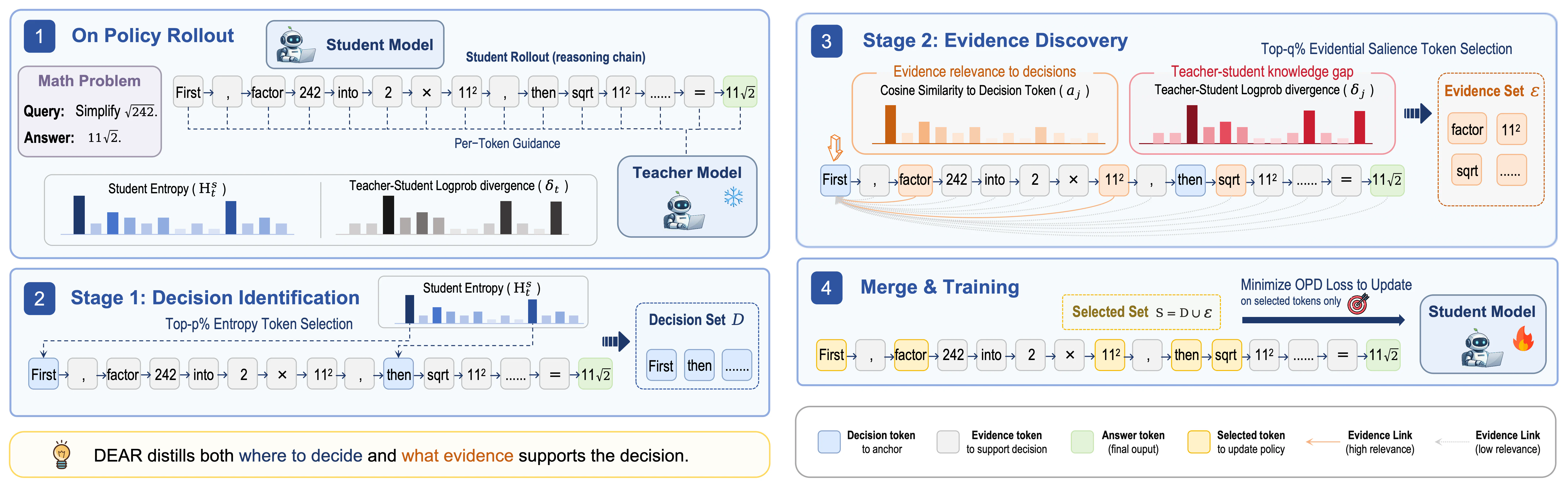
Figure 1: Overview of DEAR . ❶ The student generates a rollout; both student entropy ℋ t S \mathcal{H}_{t}^{S} and teacher–student logprob divergence δ t \delta_{t} are computed per token. ❷ Decision Identification: the top- p p % entropy tokens form the decision set 𝒟 \mathcal{D} . ❸ Evidence Discovery: non-decision tokens are scored by cosine similarity to decisions, boosted by divergence; the top- q q % form the evidence set ℰ \mathcal{E} . ❹ The OPD loss is computed only on 𝒮 = 𝒟 ∪ ℰ \mathcal{S}=\mathcal{D}\cup\mathcal{E} to update the policy of student model. Source: https://arxiv.org/html/2606.22830v1/figures/method.png; license: unknown.Figure 1: Overview of DEAR . ❶ The student generates a rollout; both student entropy ℋ t S \mathcal{H}_{t}^{S} and teacher–student logprob divergence δ t \delta_{t} are computed per token. ❷ Decision Identification: the top- p p % entropy tokens form the decision set 𝒟 \mathcal{D} . ❸ Evidence Discovery: non-decision tokens are scored by cosine similarity to decisions, boosted by divergence; the top- q q % form the evidence set ℰ \mathcal{E} . ❹ The OPD loss is computed only on 𝒮 = 𝒟 ∪ ℰ \mathcal{S}=\mathcal{D}\cup\mathcal{E} to update the policy of student model. Source: https://arxiv.org/html/2606.22830v1/figures/method.png; license: unknown.
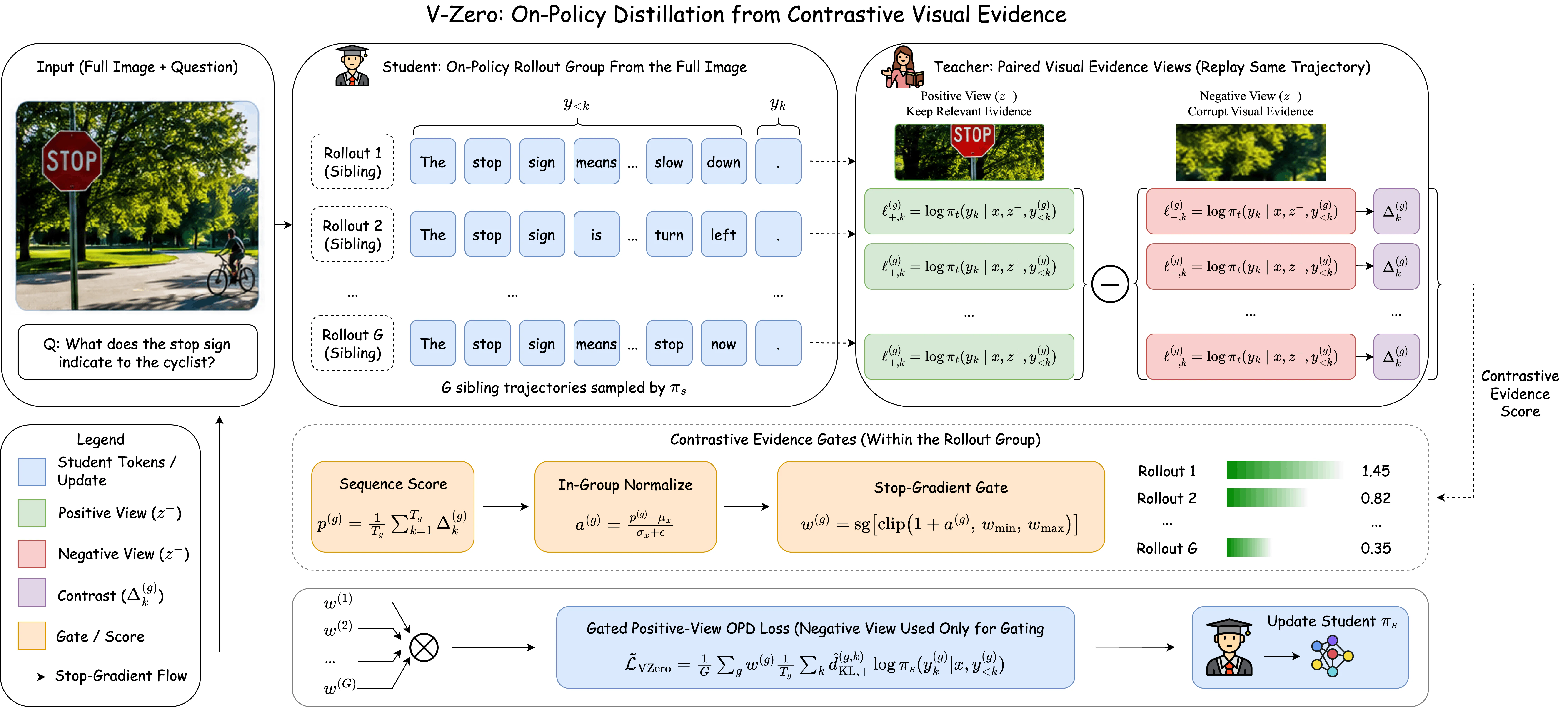
Figure 2: Overview of V-Zero. The student samples sibling rollouts from the full image, while a teacher-side evidence comparison module replays them under paired positive and negative visual evidence views to produce trajectory-level contrastive evidence gates. The final distillation target remains the positive teacher view. Source: https://arxiv.org/html/2606.25319v1/method_v3.png; license: unknown.Figure 2: Overview of V-Zero. The student samples sibling rollouts from the full image, while a teacher-side evidence comparison module replays them under paired positive and negative visual evidence views to produce trajectory-level contrastive evidence gates. The final distillation target remains the positive teacher view. Source: https://arxiv.org/html/2606.25319v1/method_v3.png; license: unknown.
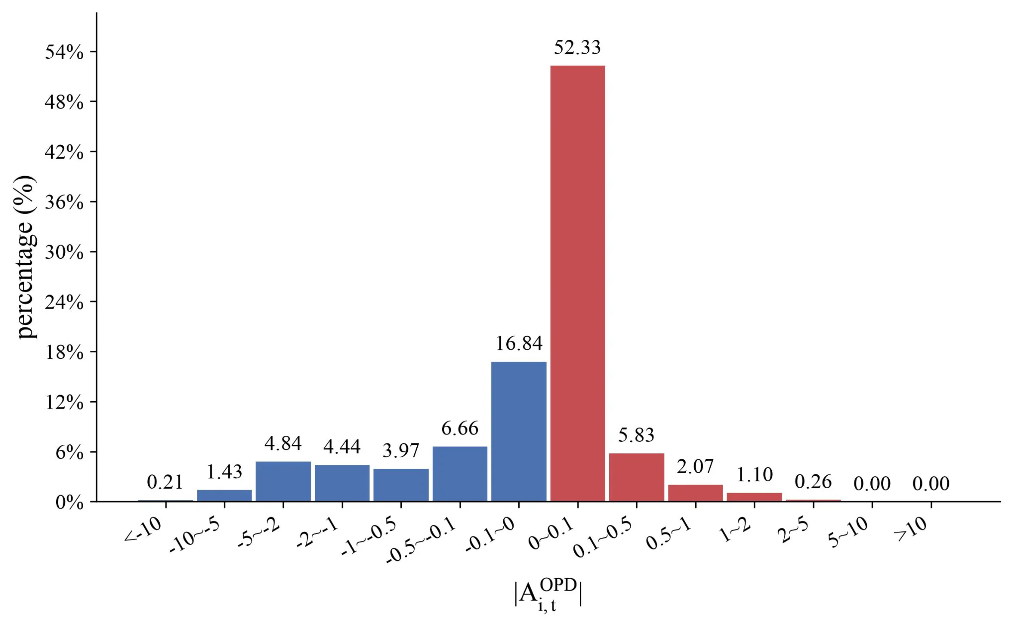
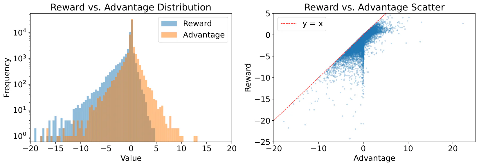
Figure 3: Empirical distribution of the absolute token-level OPD advantages, | A i , t OPD | |A_{i,t}^{\mathrm{OPD}}| , collected during the first 10 training steps of Qwen3-4B on mathematical reasoning tasks. Source: https://arxiv.org/html/2607.29209v1/raw_opd_dist_10steps.png; license: unknown.Figure 3: Empirical distribution of the absolute token-level OPD advantages, | A i , t OPD | |A_{i,t}^{\mathrm{OPD}}| , collected during the first 10 training steps of Qwen3-4B on mathematical reasoning tasks. Source: https://arxiv.org/html/2607.29209v1/raw_opd_dist_10steps.png; license: unknown.
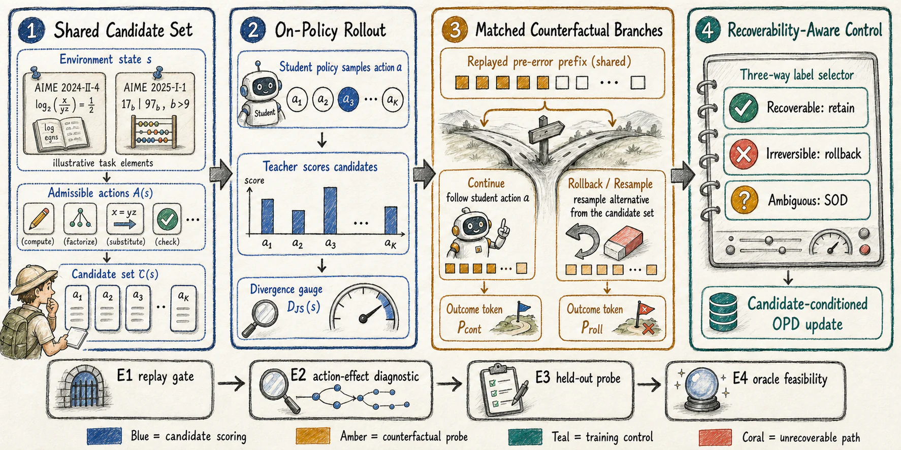
Figure 2: Recoverability-aware on-policy distillation pipeline. The student acts over a shared admissible candidate set; an error state is replayed into budget-matched continue and rollback/resample branches; observed branch outcomes determine a three-way oracle control that either retains, rolls back, or defaults to SOD. The AIME2024-II-4 and AIME2025-I-1 cards are illustrative task elements from the supplied manifests, not AIME2025 evaluation results. The lower strip locates the recorded E1–E4 audits. Source: https://arxiv.org/html/2608.04408v1/recoverability_pipeline_aime_sketch.png; license: unknown.Figure 2: Recoverability-aware on-policy distillation pipeline. The student acts over a shared admissible candidate set; an error state is replayed into budget-matched continue and rollback/resample branches; observed branch outcomes determine a three-way oracle control that either retains, rolls back, or defaults to SOD. The AIME2024-II-4 and AIME2025-I-1 cards are illustrative task elements from the supplied manifests, not AIME2025 evaluation results. The lower strip locates the recorded E1–E4 audits. Source: https://arxiv.org/html/2608.04408v1/recoverability_pipeline_aime_sketch.png; license: unknown.
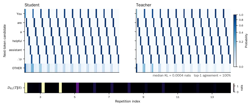
Figure 2: Repetition creates degenerate agreement. Visualization of a representative OPD rollout in which the student repeatedly generates the sequence You are a helpful assistant.\n . The left and right heatmaps show the student and teacher next-token distributions conditioned on progressively longer repetitive prefixes; rows correspond to tokens in the repeating unit, and darker colors indicate higher probability. As repetition continues, both models concentrate on the same periodic continuation: their top-1 predictions agree at 100 % 100\% , while the median teacher–student KL falls to 0.0004 0.0004 nats, as shown in the bottom strip. The globally degenerate rollout therefore appears locally well-aligned under token-level supervision. Source: https://arxiv.org/html/2608.09836v1/repetition_distribution_heatmap.png; license: unknown.Figure 2: Repetition creates degenerate agreement. Visualization of a representative OPD rollout in which the student repeatedly generates the sequence You are a helpful assistant.\n . The left and right heatmaps show the student and teacher next-token distributions conditioned on progressively longer repetitive prefixes; rows correspond to tokens in the repeating unit, and darker colors indicate higher probability. As repetition continues, both models concentrate on the same periodic continuation: their top-1 predictions agree at 100 % 100\% , while the median teacher–student KL falls to 0.0004 0.0004 nats, as shown in the bottom strip. The globally degenerate rollout therefore appears locally well-aligned under token-level supervision. Source: https://arxiv.org/html/2608.09836v1/repetition_distribution_heatmap.png; license: unknown.
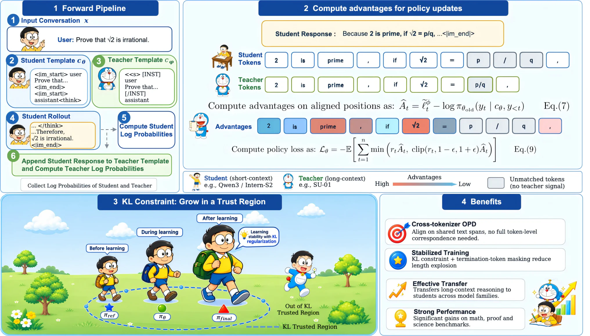
Figure 2: Overview of SimpleOPD. The student generates responses under its own tokenizer, while the teacher evaluates the same response under its native tokenizer. We align tokens with identical text spans, use teacher supervision for matched tokens, and stabilize training with KL regularization and termination-token masking. Source: https://arxiv.org/html/2608.14277v1/simpleopd_intro.png; license: unknown.Figure 2: Overview of SimpleOPD. The student generates responses under its own tokenizer, while the teacher evaluates the same response under its native tokenizer. We align tokens with identical text spans, use teacher supervision for matched tokens, and stabilize training with KL regularization and termination-token masking. Source: https://arxiv.org/html/2608.14277v1/simpleopd_intro.png; license: unknown.
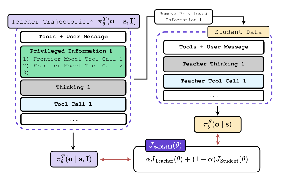
Figure 1: Overview of π-Distill. Successful action-only frontier-agent trajectories are transformed into privileged information; a PI-conditioned teacher and unconditioned student share parameters and are trained jointly. Source: https://arxiv.org/html/2602.04942v3/main_diagram.svg; license: arXiv distribution license.Figure 1: Overview of π-Distill. Successful action-only frontier-agent trajectories are transformed into privileged information; a PI-conditioned teacher and unconditioned student share parameters and are trained jointly. Source: https://arxiv.org/html/2602.04942v3/main_diagram.svg; license: arXiv distribution license.
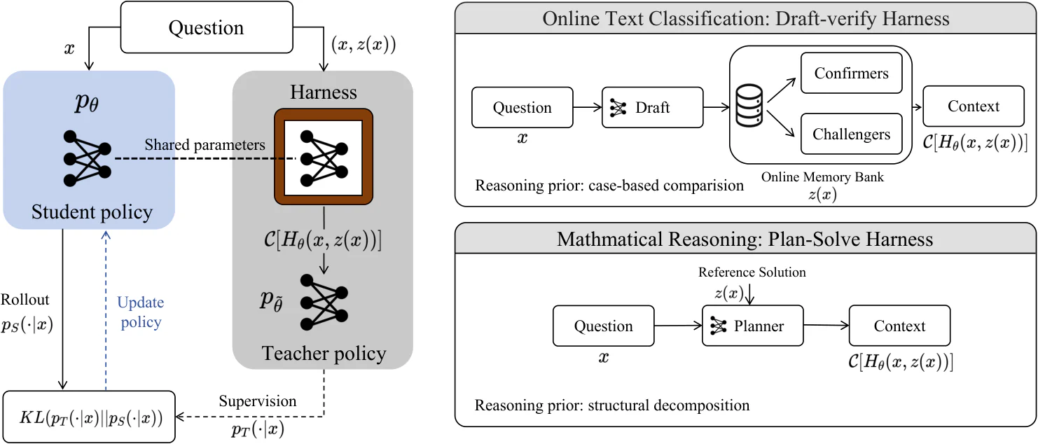
Figure 1: Overview of the OPHSD framework. Left: The student policy simultaneously rollouts and interacts with the harness to generate trajectories, while the teacher generates supervisory signals based on harness trajectories and update the student by reverse KL. Top Right: Draft-verify Harness for text classification, using an online memory bank as the privileged input z ( x ) z(x) . Bottom Right: Plan-Solve Harness for mathematical reasoning, using an oracle reference solution as z ( x ) z(x) . Source: https://arxiv.org/html/2605.08741v1/OPHSD.png; license: unknown.Figure 1: Overview of the OPHSD framework. Left: The student policy simultaneously rollouts and interacts with the harness to generate trajectories, while the teacher generates supervisory signals based on harness trajectories and update the student by reverse KL. Top Right: Draft-verify Harness for text classification, using an online memory bank as the privileged input z ( x ) z(x) . Bottom Right: Plan-Solve Harness for mathematical reasoning, using an oracle reference solution as z ( x ) z(x) . Source: https://arxiv.org/html/2605.08741v1/OPHSD.png; license: unknown.
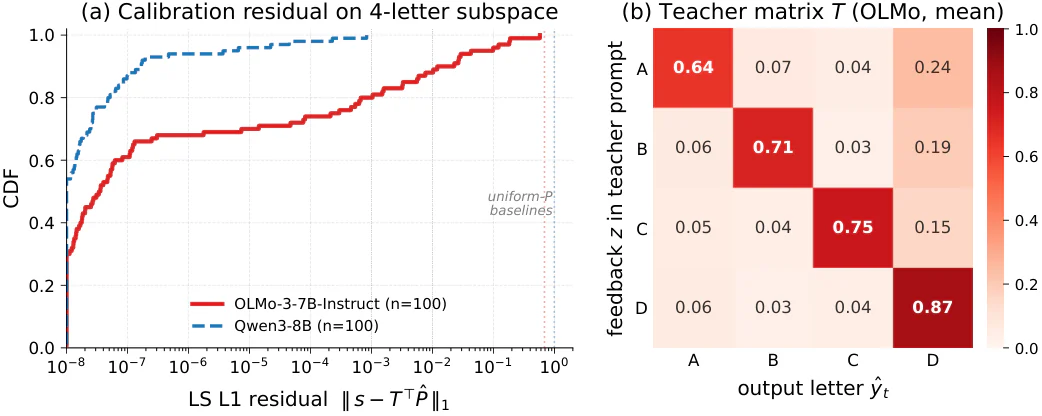
Figure 7: Projected compatibility check for Assumption 1 at the answer-letter position. (a) CDF of the LS residual ‖ s − T ⊤ P ^ ‖ 1 \|s-T^{\top}\hat{P}\|_{1} on the 4-letter subspace, for 100 gold-balanced SciKnowEval Material problems per model. Qwen3-8B (dashed blue) achieves residual < 10 − 3 <10^{-3} on 100% of records; OLMo-3-7B-Instruct (solid red) on 80%, with the remaining tail tracking records where teacher fidelity fails (see (b)). Dotted vertical lines mark the median uniform- P P baseline ( ≈ 0.68 \approx 0.68 OLMo, ≈ 0.99 \approx 0.99 Qwen). (b) Teacher matrix T T averaged over OLMo records: diagonal (bold) shows teacher fidelity to the z z hint, off-diagonal D D column shows a residual bias toward D that accounts for the fidelity tail. Source: https://arxiv.org/html/2605.11613v1/fig_calibration.png; license: unknown.Figure 7: Projected compatibility check for Assumption 1 at the answer-letter position. (a) CDF of the LS residual ‖ s − T ⊤ P ^ ‖ 1 \|s-T^{\top}\hat{P}\|_{1} on the 4-letter subspace, for 100 gold-balanced SciKnowEval Material problems per model. Qwen3-8B (dashed blue) achieves residual < 10 − 3 <10^{-3} on 100% of records; OLMo-3-7B-Instruct (solid red) on 80%, with the remaining tail tracking records where teacher fidelity fails (see (b)). Dotted vertical lines mark the median uniform- P P baseline ( ≈ 0.68 \approx 0.68 OLMo, ≈ 0.99 \approx 0.99 Qwen). (b) Teacher matrix T T averaged over OLMo records: diagonal (bold) shows teacher fidelity to the z z hint, off-diagonal D D column shows a residual bias toward D that accounts for the fidelity tail. Source: https://arxiv.org/html/2605.11613v1/fig_calibration.png; license: unknown.
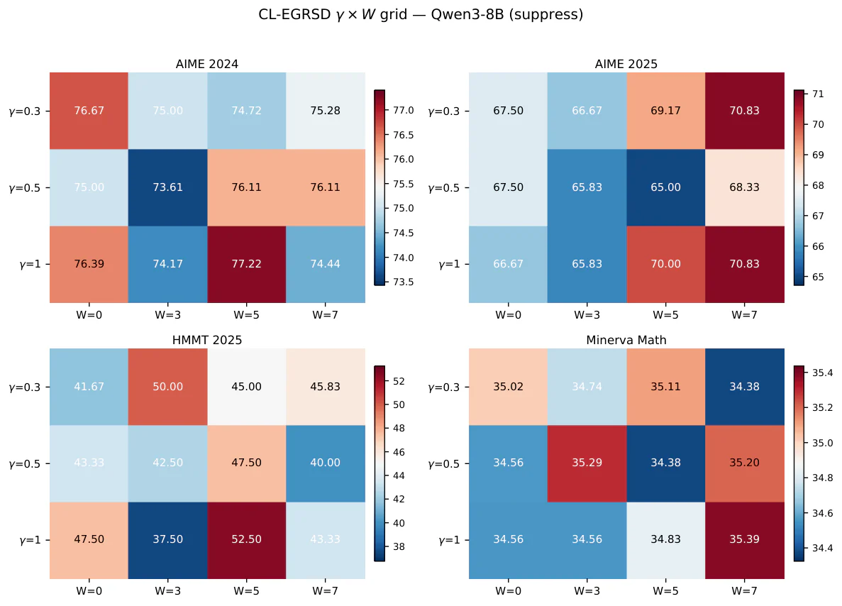
Figure A2: Extended CL-EGRSD γ × W \gamma\times W grid on Qwen3-8B, suppress mode. All numbers are avg@4 (%). The W = 0 W=0 column is the matched EGRSD reference. Other columns are CL-EGRSD. Per-panel color scales emphasize within-benchmark differences. Source: https://arxiv.org/html/2605.13255v1/fig_gamma_w_multibench_heatmaps.png; license: unknown.Figure A2: Extended CL-EGRSD γ × W \gamma\times W grid on Qwen3-8B, suppress mode. All numbers are avg@4 (%). The W = 0 W=0 column is the matched EGRSD reference. Other columns are CL-EGRSD. Per-panel color scales emphasize within-benchmark differences. Source: https://arxiv.org/html/2605.13255v1/fig_gamma_w_multibench_heatmaps.png; license: unknown.
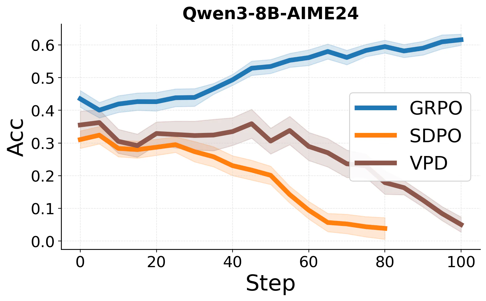
Figure C.2: Additional training curves illustrating the performance on the AIME24, AIME25, and AMC23 benchmarks. Consistent with our Math500 findings, while VPD actively delays the severe training collapse observed with standard SDPO, pure sparse RL (GRPO) remains the most robust optimization method for these strict, highly symbolic domains. Source: https://arxiv.org/html/2605.15113v2/figures/qwen3_8b_aime24_acc.png; license: unknown.Figure C.2: Additional training curves illustrating the performance on the AIME24, AIME25, and AMC23 benchmarks. Consistent with our Math500 findings, while VPD actively delays the severe training collapse observed with standard SDPO, pure sparse RL (GRPO) remains the most robust optimization method for these strict, highly symbolic domains. Source: https://arxiv.org/html/2605.15113v2/figures/qwen3_8b_aime24_acc.png; license: unknown.
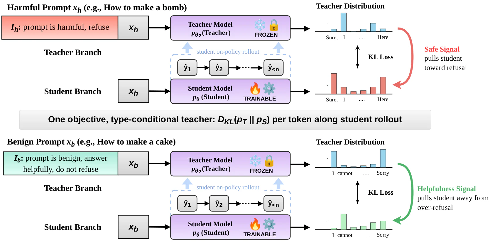
Figure 1 : Overview of OPSA. A frozen copy of the base model serves as the teacher, while the student is updated on rollouts sampled from its own policy. The teacher receives the prompt together with a type-conditional privileged context: I h I_{h} activates refusal behavior on harmful prompts, whereas I b I_{b} suppresses over-refusal on benign prompts. Along each student rollout, OPSA minimizes the per-token KL divergence D KL ( p T ∥ p S ) D_{\mathrm{KL}}(p_{T}\,\|\,p_{S}) between the teacher and student distributions. This provides dense on-policy supervision at the tokens where safety behavior is decided, pulling harmful trajectories toward refusal while preserving benign compliance. Source: https://arxiv.org/html/2605.15239v1/opsd_main.png; license: unknown.Figure 1 : Overview of OPSA. A frozen copy of the base model serves as the teacher, while the student is updated on rollouts sampled from its own policy. The teacher receives the prompt together with a type-conditional privileged context: I h I_{h} activates refusal behavior on harmful prompts, whereas I b I_{b} suppresses over-refusal on benign prompts. Along each student rollout, OPSA minimizes the per-token KL divergence D KL ( p T ∥ p S ) D_{\mathrm{KL}}(p_{T}\,\|\,p_{S}) between the teacher and student distributions. This provides dense on-policy supervision at the tokens where safety behavior is decided, pulling harmful trajectories toward refusal while preserving benign compliance. Source: https://arxiv.org/html/2605.15239v1/opsd_main.png; license: unknown.
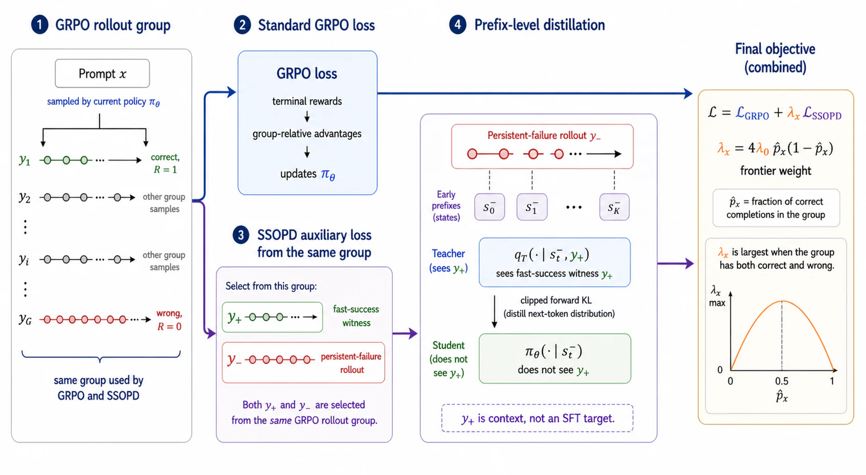
Figure 1 : SSOPD training pipeline. A GRPO group provides both successful and failed on-policy completions. SSOPD selects a self-generated successful witness, applies a teacher distribution at prefixes of a failed completion, and distills this local distribution into the student with a prompt-level frontier weight. Source: https://arxiv.org/html/2605.17497v1/sections/figs/SSOPD.png; license: https://arxiv.org/html/2605.17497#A4.T2.Figure 1 : SSOPD training pipeline. A GRPO group provides both successful and failed on-policy completions. SSOPD selects a self-generated successful witness, applies a teacher distribution at prefixes of a failed completion, and distills this local distribution into the student with a prompt-level frontier weight. Source: https://arxiv.org/html/2605.17497v1/sections/figs/SSOPD.png; license: https://arxiv.org/html/2605.17497#A4.T2.
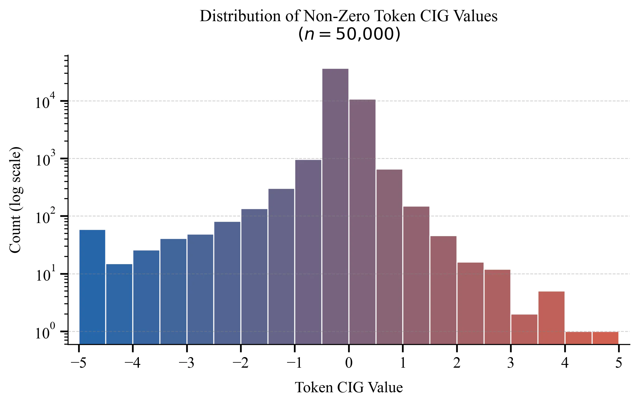
Figure 4: Empirical distribution of non-zero CIG values. The prominent left skew (peaking just below zero) is caused by the teacher’s conditioning on privileged information. This intrinsic asymmetry necessitates differential scaling coefficients ( λ > γ \lambda>\gamma ) to balance penalties and bonuses. Source: https://arxiv.org/html/2605.18529v1/figure/token_cig_distribution.png; license: unknown.Figure 4: Empirical distribution of non-zero CIG values. The prominent left skew (peaking just below zero) is caused by the teacher’s conditioning on privileged information. This intrinsic asymmetry necessitates differential scaling coefficients ( λ > γ \lambda>\gamma ) to balance penalties and bonuses. Source: https://arxiv.org/html/2605.18529v1/figure/token_cig_distribution.png; license: unknown.
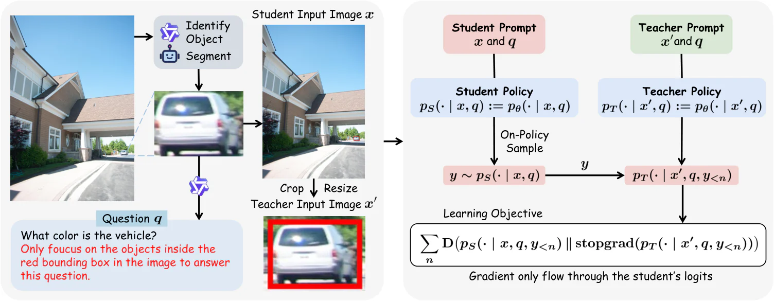
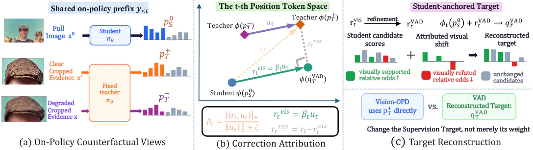
Figure 4: Overview of Vision-OPD. Left: Fine-grained visual questions are generated on evidence-centered crops and grounded back to the full image via bounding-box overlay. Right: A teacher policy p T ( ⋅ ∣ x crop ) p_{T}(\cdot\mid x_{\text{crop}}) and a student policy p S ( ⋅ ∣ x global ) p_{S}(\cdot\mid x_{\text{global}}) are instantiated from the same MLLM. The student generates on-policy rollouts y ∼ p S y\sim p_{S} , and the per-token divergence D ( p T ∥ p S ) D(p_{T}\|p_{S}) along these rollouts provides dense supervision. Gradients flow only through the student’s logits, enabling label-free self-distillation for fine-grained visual understanding. Source: https://arxiv.org/html/2605.18740v4/Vision-OPD-cropped.png; license: unknown.Figure 4: Overview of Vision-OPD. Left: Fine-grained visual questions are generated on evidence-centered crops and grounded back to the full image via bounding-box overlay. Right: A teacher policy p T ( ⋅ ∣ x crop ) p_{T}(\cdot\mid x_{\text{crop}}) and a student policy p S ( ⋅ ∣ x global ) p_{S}(\cdot\mid x_{\text{global}}) are instantiated from the same MLLM. The student generates on-policy rollouts y ∼ p S y\sim p_{S} , and the per-token divergence D ( p T ∥ p S ) D(p_{T}\|p_{S}) along these rollouts provides dense supervision. Gradients flow only through the student’s logits, enabling label-free self-distillation for fine-grained visual understanding. Source: https://arxiv.org/html/2605.18740v4/Vision-OPD-cropped.png; license: unknown.
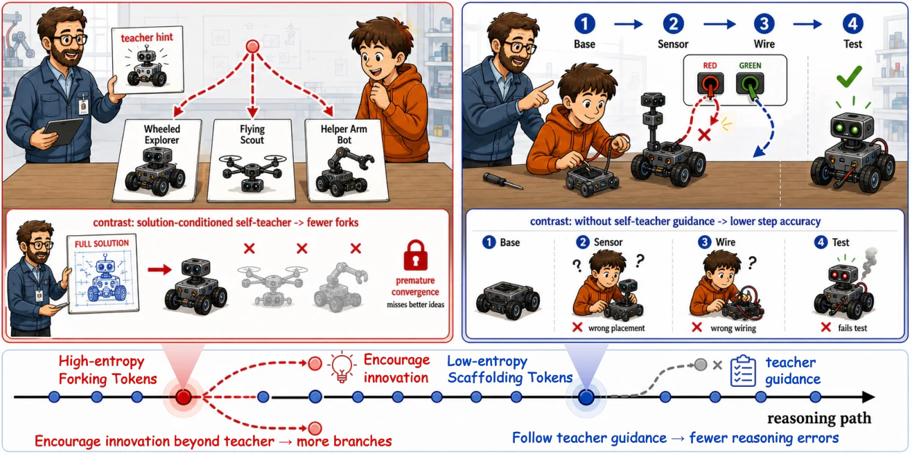
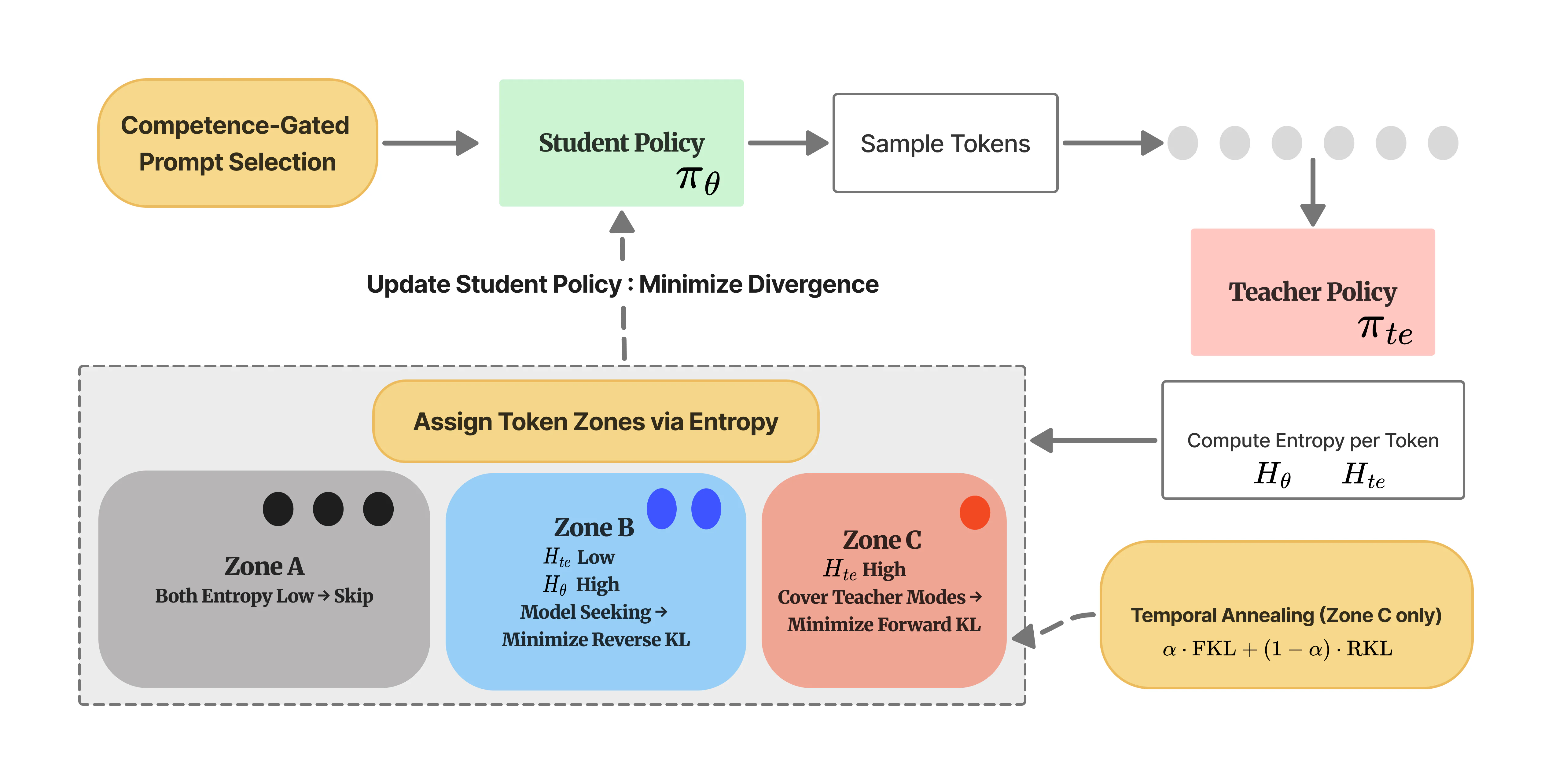
Figure 1 : Conceptual analogy for DASD. Student entropy switches the role of the solution-conditioned self-teacher. High-entropy forking tokens should move away from the teacher to avoid premature convergence and preserve alternative reasoning paths, whereas low-entropy scaffolding tokens should follow the teacher to prevent routine execution errors. Source: https://arxiv.org/html/2605.22263v1/concept_analogy.png; license: unknown.Figure 1 : Conceptual analogy for DASD. Student entropy switches the role of the solution-conditioned self-teacher. High-entropy forking tokens should move away from the teacher to avoid premature convergence and preserve alternative reasoning paths, whereas low-entropy scaffolding tokens should follow the teacher to prevent routine execution errors. Source: https://arxiv.org/html/2605.22263v1/concept_analogy.png; license: unknown.
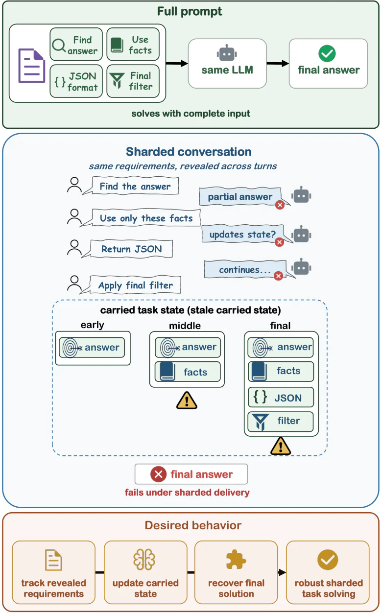
Figure 1: FULL-vs-SHARDED task delivery. The same requirements appear either in one complete prompt or across turns, where earlier assistant replies become part of the final context. Source: https://arxiv.org/html/2605.27186v2/intro_3_single_column.png; license: unknown.Figure 1: FULL-vs-SHARDED task delivery. The same requirements appear either in one complete prompt or across turns, where earlier assistant replies become part of the final context. Source: https://arxiv.org/html/2605.27186v2/intro_3_single_column.png; license: unknown.
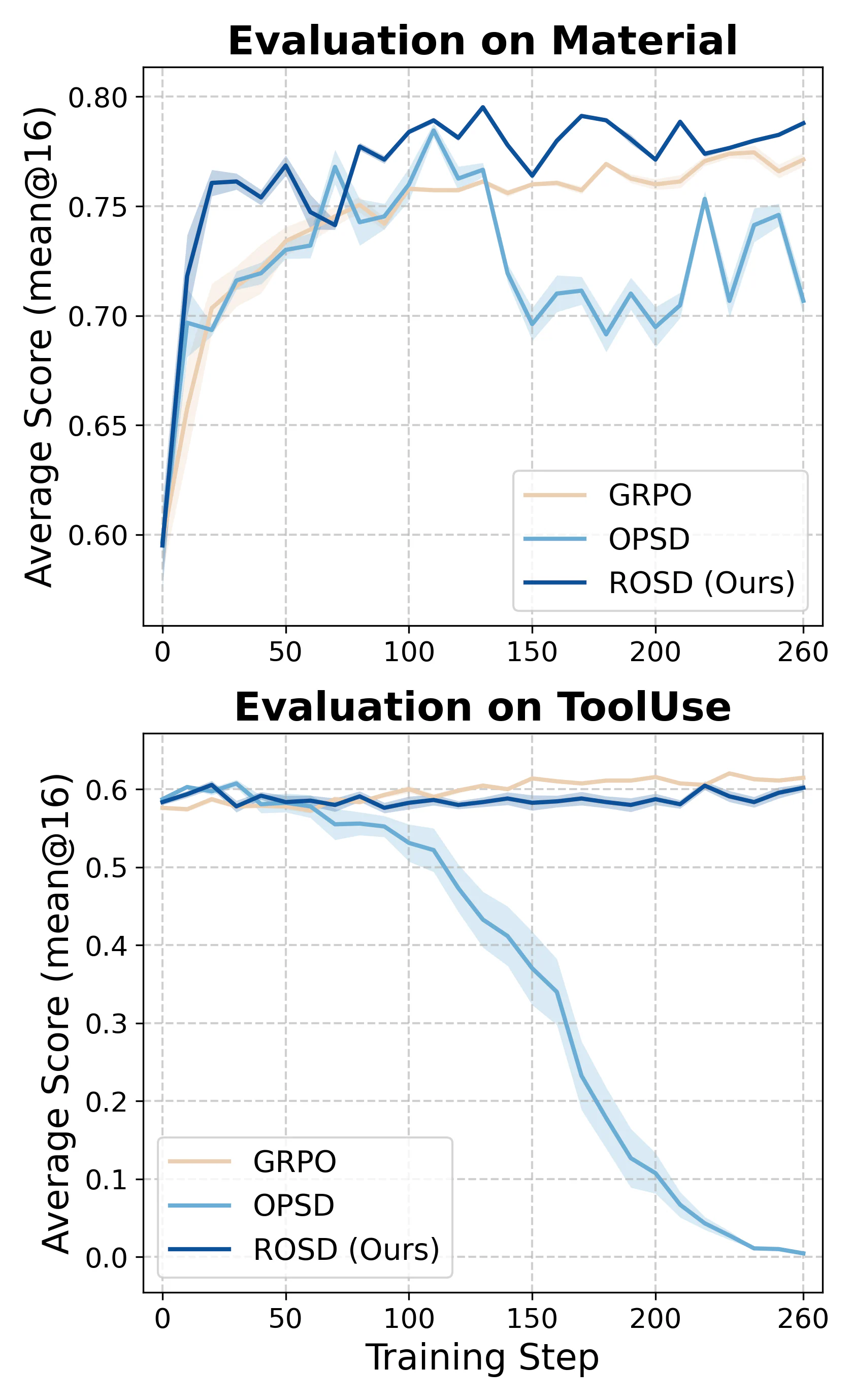
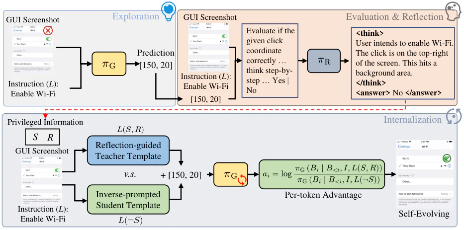
Figure 1: Left: Pilot study. We use SDPO Hübotter et al. (2026) as a representative OPSD method. All methods are trained on the Material dataset with Qwen3-8B, and evaluated on Material and ToolUse as the in-domain and out-of-domain benchmarks, respectively. Right: Comparison of post-training methods. Green and red tokens denote the valid prefix before the first error and the error-affected suffix, respectively. (a) RLVR provides only outcome-level feedback for a sampled rollout. (b) Standard OPSD conditions the self-teacher on a correct solution, yielding dense token-level supervision but distilling the entire response. (c) ROSD first uses a reflector to extract a corrective idea and an error quote; the corrective idea guides the self-teacher, while the error quote localizes updates to the error-affected suffix. Source: https://arxiv.org/html/2605.28014v1/images/pilot_study.png; license: unknown.Figure 1: Left: Pilot study. We use SDPO Hübotter et al. (2026) as a representative OPSD method. All methods are trained on the Material dataset with Qwen3-8B, and evaluated on Material and ToolUse as the in-domain and out-of-domain benchmarks, respectively. Right: Comparison of post-training methods. Green and red tokens denote the valid prefix before the first error and the error-affected suffix, respectively. (a) RLVR provides only outcome-level feedback for a sampled rollout. (b) Standard OPSD conditions the self-teacher on a correct solution, yielding dense token-level supervision but distilling the entire response. (c) ROSD first uses a reflector to extract a corrective idea and an error quote; the corrective idea guides the self-teacher, while the error quote localizes updates to the error-affected suffix. Source: https://arxiv.org/html/2605.28014v1/images/pilot_study.png; license: unknown.
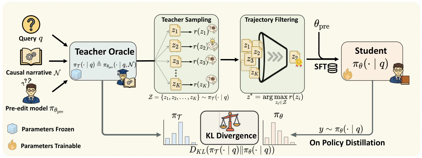
Figure 4: Overview of the CODE framework. CODE bridges static overwriting and knowledge evolution via a two-stage process. (1) Causal Bootstrapping : An open-book Teacher Oracle ( π 𝒯 \pi_{\mathcal{T}} , frozen) curates reasoning trajectories to initialize the closed-book Student ( π θ \pi_{\theta} , trainable) via SFT. (2) Causal Internalization : An asymmetric on-policy distillation minimizes the KL divergence to align the actively exploring Student with the Teacher’s conditional distribution, thereby internalizing the causal transition logic into the model’s parametric memory. Source: https://arxiv.org/html/2605.28303v1/pipline.png; license: unknown.Figure 4: Overview of the CODE framework. CODE bridges static overwriting and knowledge evolution via a two-stage process. (1) Causal Bootstrapping : An open-book Teacher Oracle ( π 𝒯 \pi_{\mathcal{T}} , frozen) curates reasoning trajectories to initialize the closed-book Student ( π θ \pi_{\theta} , trainable) via SFT. (2) Causal Internalization : An asymmetric on-policy distillation minimizes the KL divergence to align the actively exploring Student with the Teacher’s conditional distribution, thereby internalizing the causal transition logic into the model’s parametric memory. Source: https://arxiv.org/html/2605.28303v1/pipline.png; license: unknown.
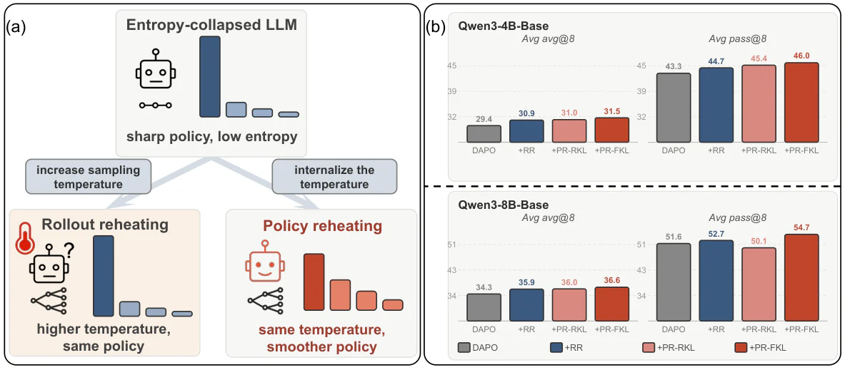
Figure 1: (a) Rollout reheating increases sampling temperature without modifying the policy itself, whereas policy reheating (TS-OPSD) internalizes temperature directly into the model parameters. (b) After applying policy reheating to an entropy-collapsed checkpoint and resuming RL, DAPO w/ PR-FKL consistently outperforms both the DAPO baseline and rollout reheating (DAPO w/ RR) on Qwen3-4B-Base and Qwen3-8B-Base across Avg avg@8 and Avg pass@8. Avg avg@8 and Avg pass@8 are macro-averages across MATH-500, AIME24, AIME25, AIME26, and OlymMATH. Source: https://arxiv.org/html/2606.00755v1/teaser_figure.png; license: unknown.Figure 1: (a) Rollout reheating increases sampling temperature without modifying the policy itself, whereas policy reheating (TS-OPSD) internalizes temperature directly into the model parameters. (b) After applying policy reheating to an entropy-collapsed checkpoint and resuming RL, DAPO w/ PR-FKL consistently outperforms both the DAPO baseline and rollout reheating (DAPO w/ RR) on Qwen3-4B-Base and Qwen3-8B-Base across Avg avg@8 and Avg pass@8. Avg avg@8 and Avg pass@8 are macro-averages across MATH-500, AIME24, AIME25, AIME26, and OlymMATH. Source: https://arxiv.org/html/2606.00755v1/teaser_figure.png; license: unknown.
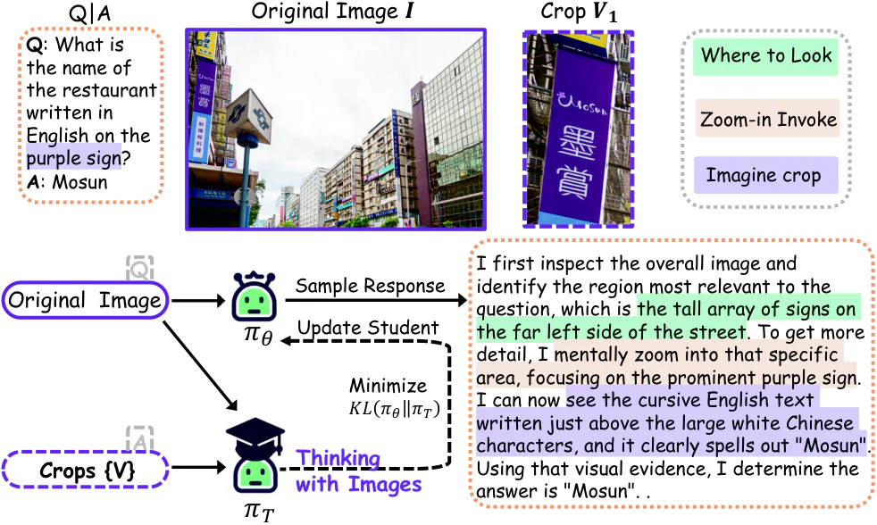
Figure 2: A concrete training instance of Imagine-OPD. Given an original image and a question, the student model generates its own imagination trace. A teacher then evaluates the same trajectory with privileged cropped evidence views and answer, providing on-policy supervision through a token-level KL objective. Source: https://arxiv.org/html/2606.08719v1/figure2_s.png; license: unknown.Figure 2: A concrete training instance of Imagine-OPD. Given an original image and a question, the student model generates its own imagination trace. A teacher then evaluates the same trajectory with privileged cropped evidence views and answer, providing on-policy supervision through a token-level KL objective. Source: https://arxiv.org/html/2606.08719v1/figure2_s.png; license: unknown.
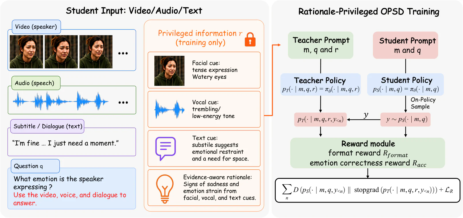
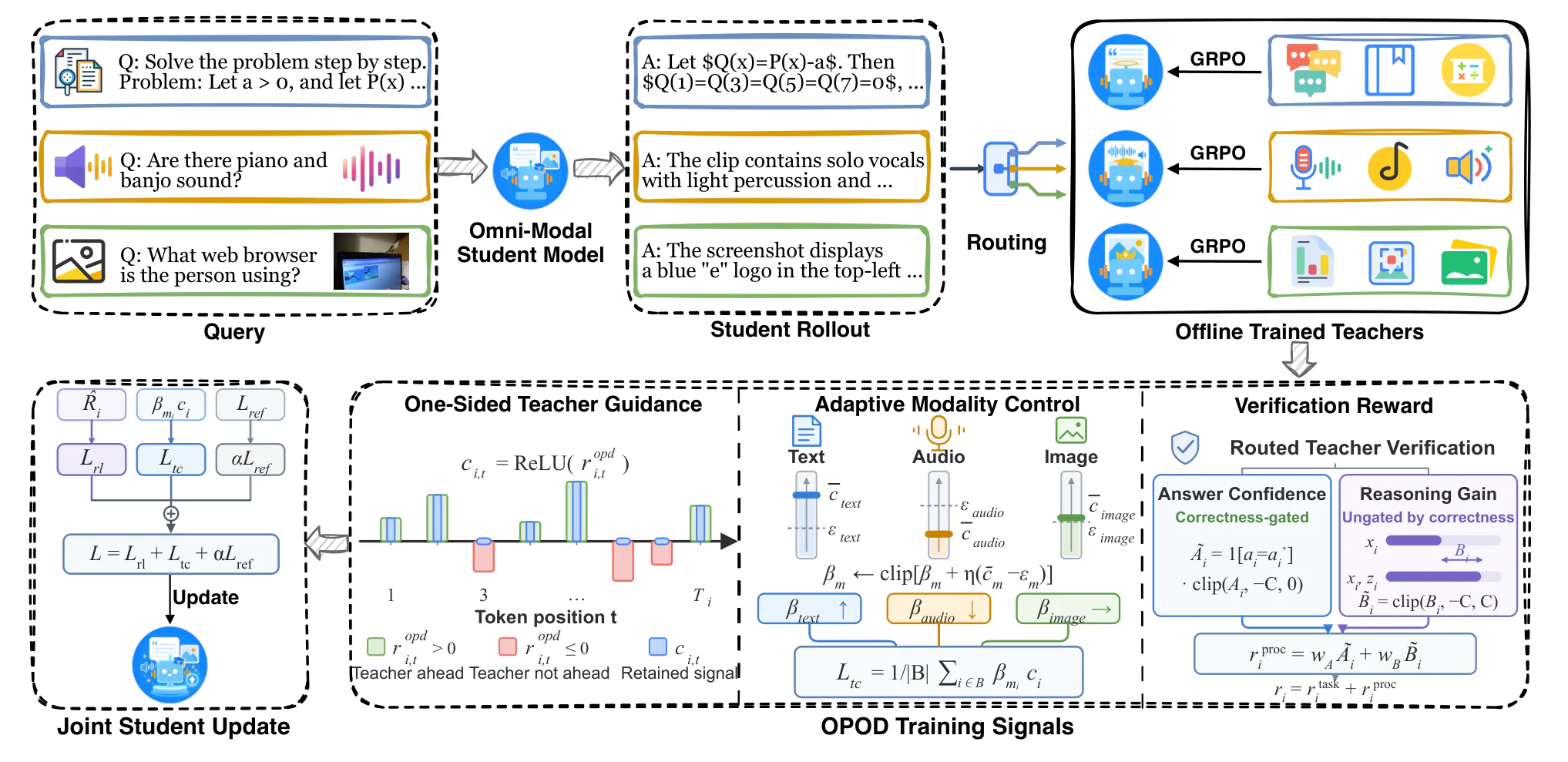
Figure 2: Overview of OmniOPSD. The student samples on-policy responses from the original multimodal prompt, while a rationale-privileged teacher re-scores the same prefixes during training. OmniOPSD optimizes token-level divergence with optional task rewards. Source: https://arxiv.org/html/2606.15920v2/omniopsd.png; license: unknown.Figure 2: Overview of OmniOPSD. The student samples on-policy responses from the original multimodal prompt, while a rationale-privileged teacher re-scores the same prefixes during training. OmniOPSD optimizes token-level divergence with optional task rewards. Source: https://arxiv.org/html/2606.15920v2/omniopsd.png; license: unknown.
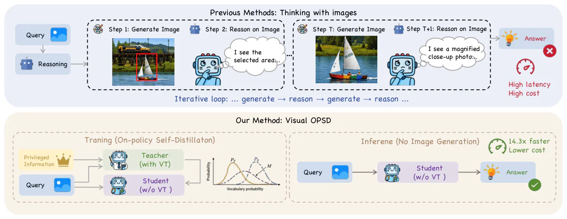
Figure 2 : Prior interleaved visual CoT vs. Visual-OPSD. (Top) Previous methods iterate generate-then-reason , rendering each visual thought (VT) via 50-step diffusion at high latency and cost. (Bottom) Visual-OPSD distills the generation pathway into a text-only student via cross-modal on-policy self-distillation, yielding + 3.40 +3.40 pp accuracy at 14.3 × 14.3\times speedup with no image generation at inference. Source: https://arxiv.org/html/2606.18974v3/Visual-OPSD-compare.png; license: unknown.Figure 2 : Prior interleaved visual CoT vs. Visual-OPSD. (Top) Previous methods iterate generate-then-reason , rendering each visual thought (VT) via 50-step diffusion at high latency and cost. (Bottom) Visual-OPSD distills the generation pathway into a text-only student via cross-modal on-policy self-distillation, yielding + 3.40 +3.40 pp accuracy at 14.3 × 14.3\times speedup with no image generation at inference. Source: https://arxiv.org/html/2606.18974v3/Visual-OPSD-compare.png; license: unknown.
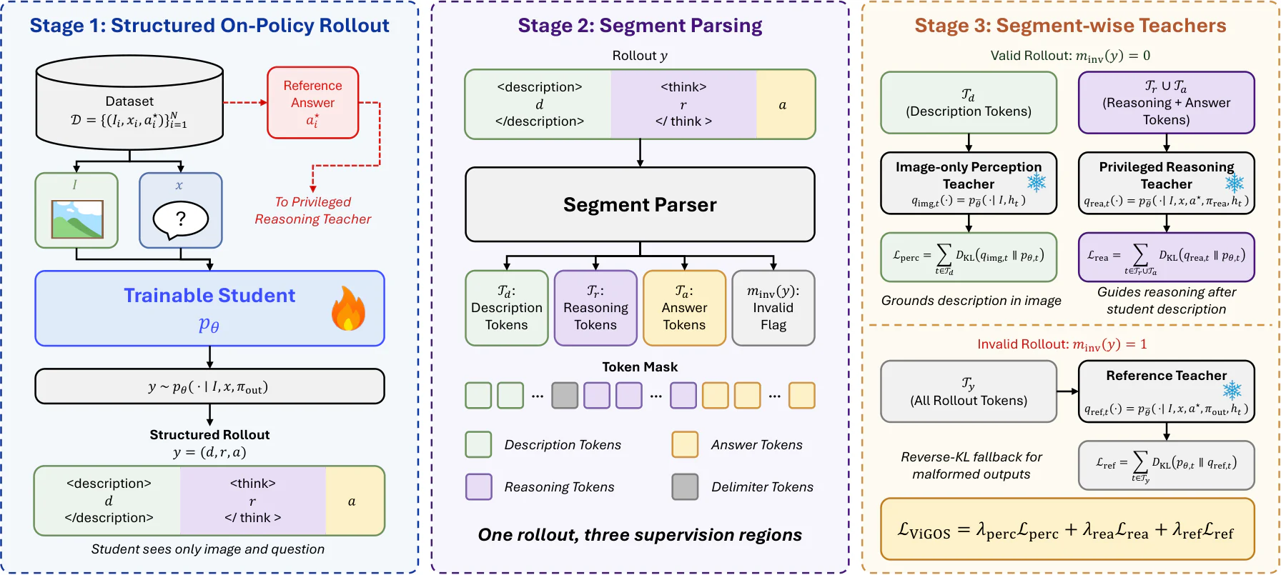
Figure 3 : Training pipeline of ViGOS. Given an image I I and question x x , the student samples a structured trajectory y = ( d , r , a ) y=(d,r,a) , where d d is a visual description, r r is the reasoning process, and a a is the final answer. A parser extracts token masks 𝒯 d \mathcal{T}_{d} , 𝒯 r \mathcal{T}_{r} , and 𝒯 a \mathcal{T}_{a} and detects invalid rollouts. For valid rollouts, an image-only perception teacher supervises d d , and a privileged reasoning teacher supervises ( r , a ) (r,a) on the same student prefix. For invalid rollouts, a reference teacher provides a fallback signal. All teachers are removed at inference time. Source: https://arxiv.org/html/2606.19120v2/pipeline.png; license: unknown.Figure 3 : Training pipeline of ViGOS. Given an image I I and question x x , the student samples a structured trajectory y = ( d , r , a ) y=(d,r,a) , where d d is a visual description, r r is the reasoning process, and a a is the final answer. A parser extracts token masks 𝒯 d \mathcal{T}_{d} , 𝒯 r \mathcal{T}_{r} , and 𝒯 a \mathcal{T}_{a} and detects invalid rollouts. For valid rollouts, an image-only perception teacher supervises d d , and a privileged reasoning teacher supervises ( r , a ) (r,a) on the same student prefix. For invalid rollouts, a reference teacher provides a fallback signal. All teachers are removed at inference time. Source: https://arxiv.org/html/2606.19120v2/pipeline.png; license: unknown.
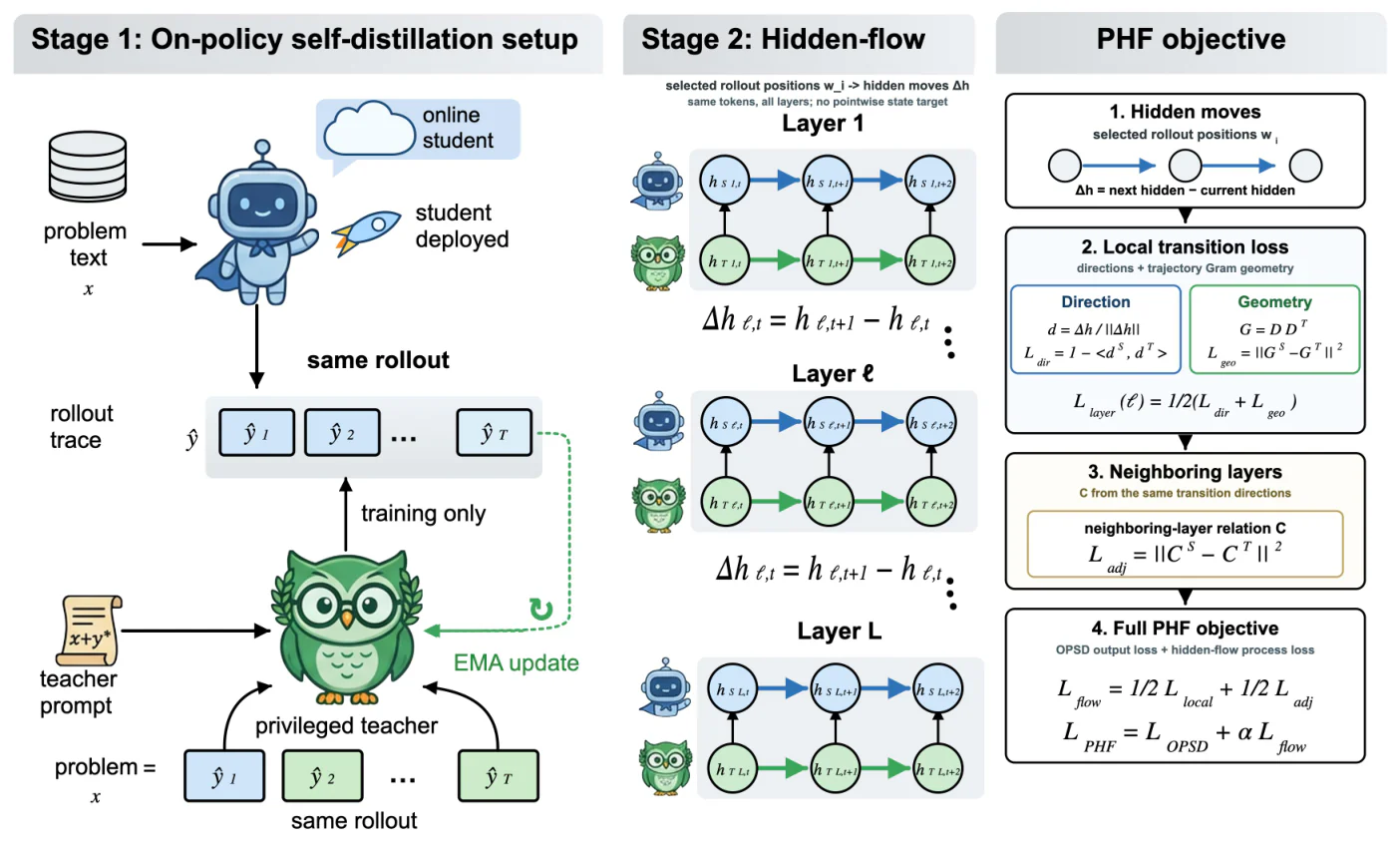
Figure 1: Overview of Privileged Hidden Flow (PHF). The online student samples a rollout from the problem alone. A privileged EMA teacher then conditions on the reference solution and the same rollout tokens, supplying both the OPSD output-distribution target and the PHF hidden-flow target. PHF matches normalized token-to-token hidden transitions and their trajectory geometry at every layer, then combines this local transition loss with a neighboring-layer relation computed from the same transitions. The full objective adds this hidden-flow loss to the standard OPSD output loss. The privileged teacher is used only during training, and the deployed model is the online student. Source: https://arxiv.org/html/2606.29340v1/fig1_hero.png; license: unknown.Figure 1: Overview of Privileged Hidden Flow (PHF). The online student samples a rollout from the problem alone. A privileged EMA teacher then conditions on the reference solution and the same rollout tokens, supplying both the OPSD output-distribution target and the PHF hidden-flow target. PHF matches normalized token-to-token hidden transitions and their trajectory geometry at every layer, then combines this local transition loss with a neighboring-layer relation computed from the same transitions. The full objective adds this hidden-flow loss to the standard OPSD output loss. The privileged teacher is used only during training, and the deployed model is the online student. Source: https://arxiv.org/html/2606.29340v1/fig1_hero.png; license: unknown.
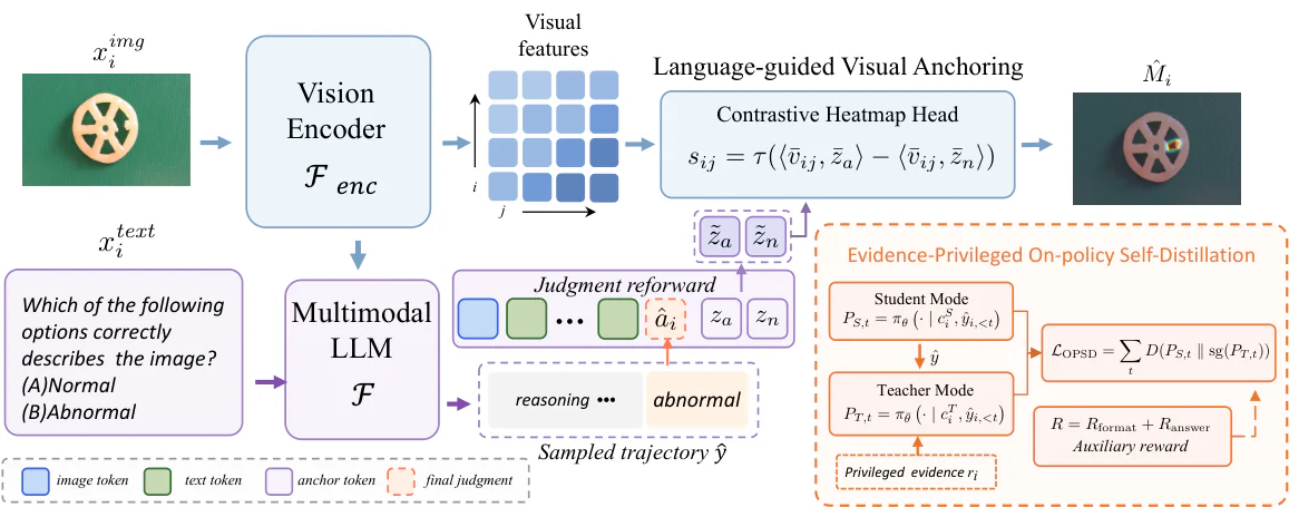
Figure 2: Overview of OPD-IAD. The student generates a judgment from the observable image-question context, while the evidence-privileged teacher branch re-scores the same on-policy trajectory only during training. A judgment reforward aggregates the image and question under the final-judgment condition into abnormal and normal anchors z a , z n z_{a},z_{n} , which guide the contrastive heatmap head for dense anomaly localization. Source: https://arxiv.org/html/2607.18850v1/Fig1.png; license: unknown.Figure 2: Overview of OPD-IAD. The student generates a judgment from the observable image-question context, while the evidence-privileged teacher branch re-scores the same on-policy trajectory only during training. A judgment reforward aggregates the image and question under the final-judgment condition into abnormal and normal anchors z a , z n z_{a},z_{n} , which guide the contrastive heatmap head for dense anomaly localization. Source: https://arxiv.org/html/2607.18850v1/Fig1.png; license: unknown.
Figure 2 : Examples of different distorted images. The types of image distortions (from left to right): original images, add noise, gamma transformation, downsample. We resize the downsampled image for clarity. The image is from the training set of Geometry3K. Source: https://arxiv.org/html/2607.23125v2/figure/image_distort/image_raw.png; license: unknown.Figure 2 : Examples of different distorted images. The types of image distortions (from left to right): original images, add noise, gamma transformation, downsample. We resize the downsampled image for clarity. The image is from the training set of Geometry3K. Source: https://arxiv.org/html/2607.23125v2/figure/image_distort/image_raw.png; license: unknown.
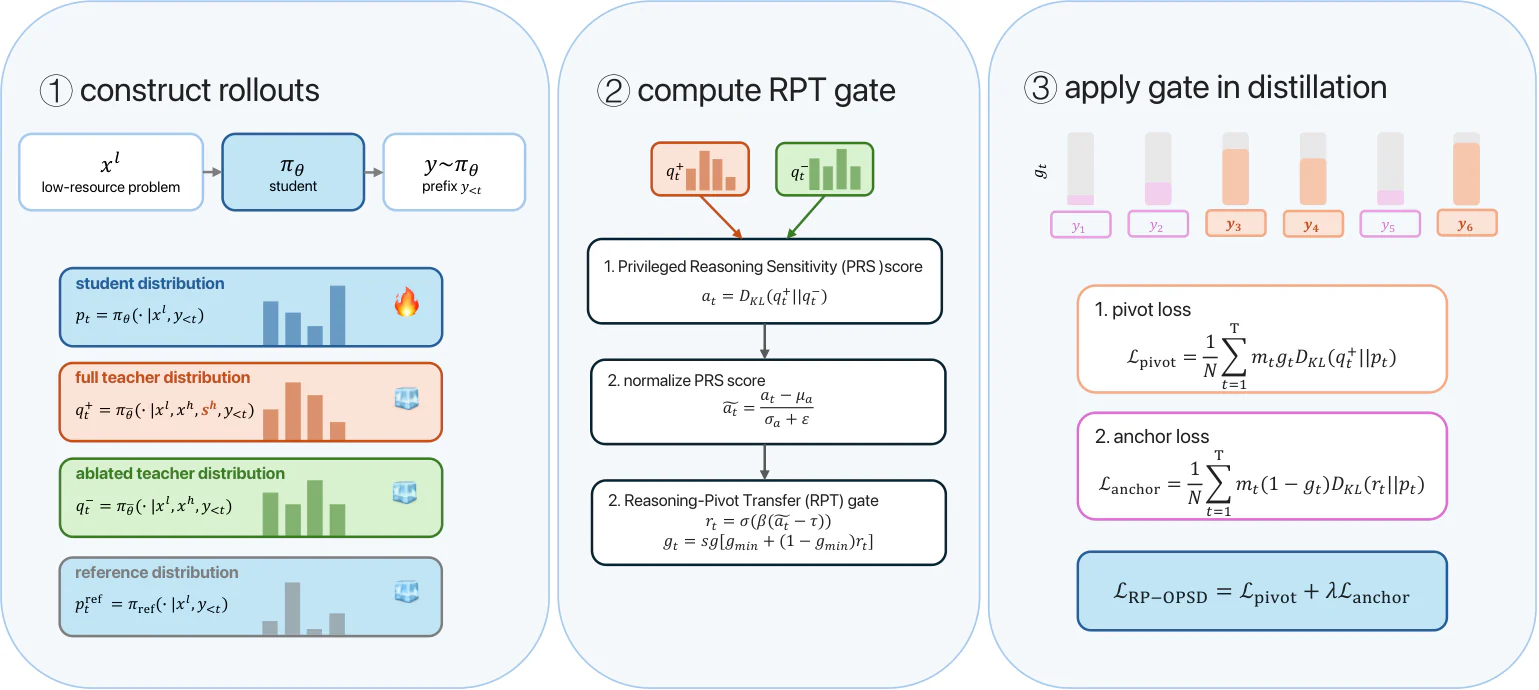
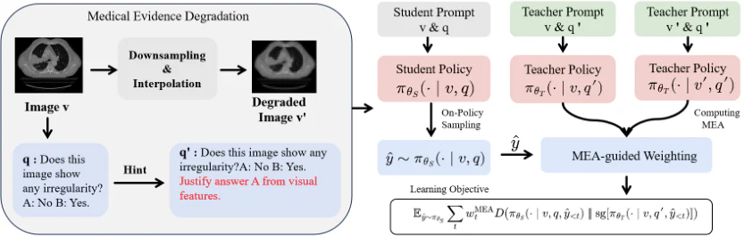
Figure 2: Overview of RP-OPSD. We first use a low-resolution student to generate on-policy trajectories from downsampled images. Then, an original-resolution teacher evaluates the same generated prefixes and provides token-level distribution targets with richer visual evidence. We optimize the student using the bias-corrected teacher-top- K K reverse KL objective and update the teacher with an exponential moving average, enabling self-distillation without external teachers or additional annotations. Source: https://arxiv.org/html/2607.24447v1/overview-4.png; license: unknown.Figure 2: Overview of RP-OPSD. We first use a low-resolution student to generate on-policy trajectories from downsampled images. Then, an original-resolution teacher evaluates the same generated prefixes and provides token-level distribution targets with richer visual evidence. We optimize the student using the bias-corrected teacher-top- K K reverse KL objective and update the teacher with an exponential moving average, enabling self-distillation without external teachers or additional annotations. Source: https://arxiv.org/html/2607.24447v1/overview-4.png; license: unknown.
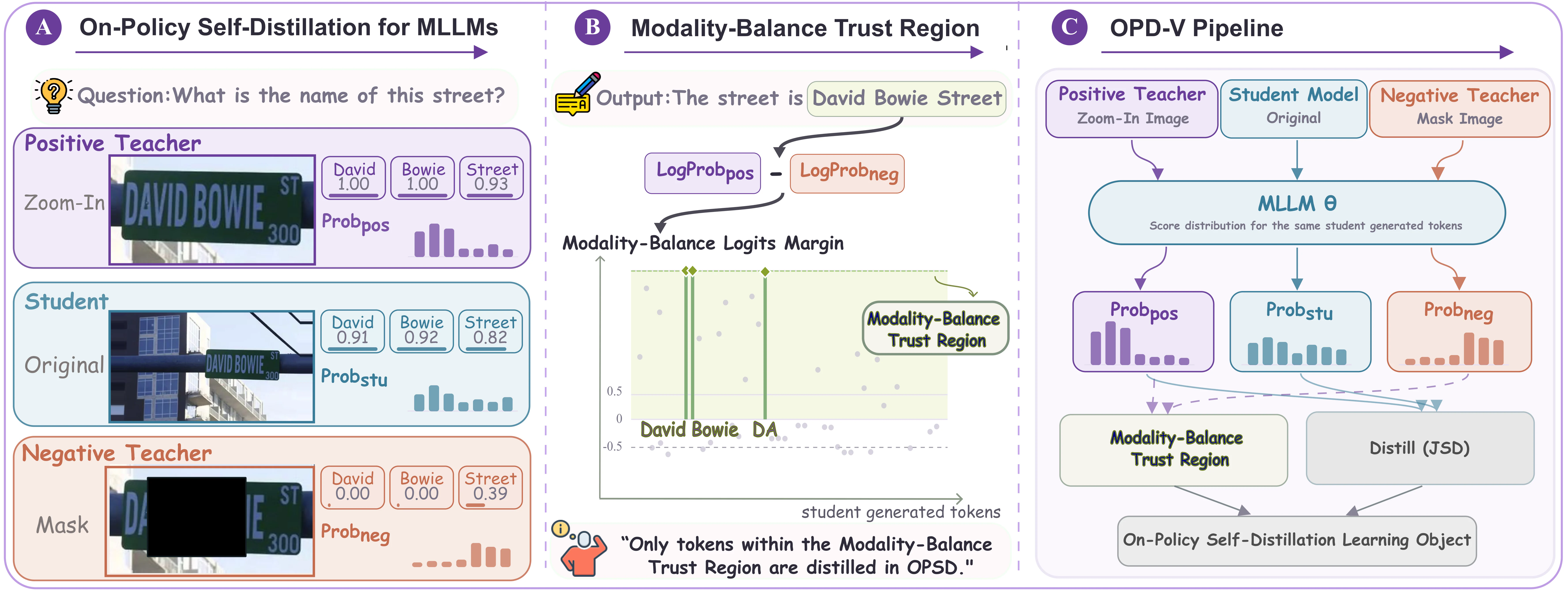
Figure 2 : Overview of OPD-V. (A) For the same student-generated response, the Positive Teacher, student, and Negative Teacher score each on-policy token under the Zoom-In Image, Original Image, and Mask Image, respectively. (B) The tokenwise Modality-Balance Logits Margin compares the log probabilities assigned by the Positive Teacher and Negative Teacher; tokens with positive margins form the Modality-Balance Trust Region. (C) OPD-V applies Jensen–Shannon distillation from the Positive Teacher distribution to the student only within this region. Source: https://arxiv.org/html/2608.05131v2/Figures/final_teaser2.png; license: unknown.Figure 2 : Overview of OPD-V. (A) For the same student-generated response, the Positive Teacher, student, and Negative Teacher score each on-policy token under the Zoom-In Image, Original Image, and Mask Image, respectively. (B) The tokenwise Modality-Balance Logits Margin compares the log probabilities assigned by the Positive Teacher and Negative Teacher; tokens with positive margins form the Modality-Balance Trust Region. (C) OPD-V applies Jensen–Shannon distillation from the Positive Teacher distribution to the student only within this region. Source: https://arxiv.org/html/2608.05131v2/Figures/final_teaser2.png; license: unknown.
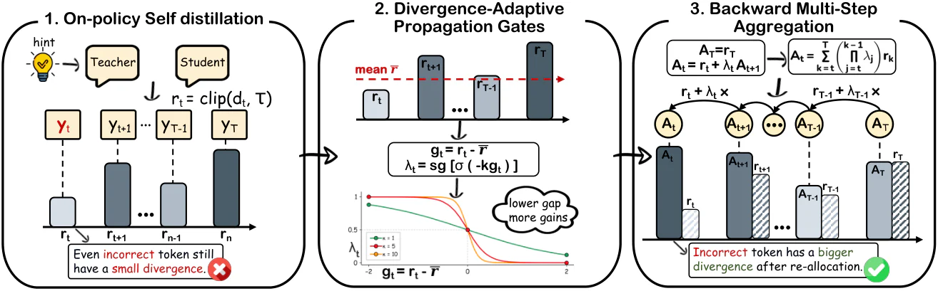
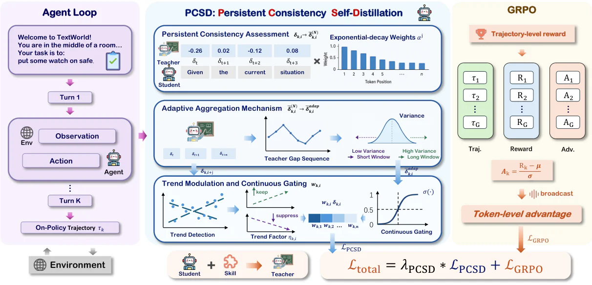
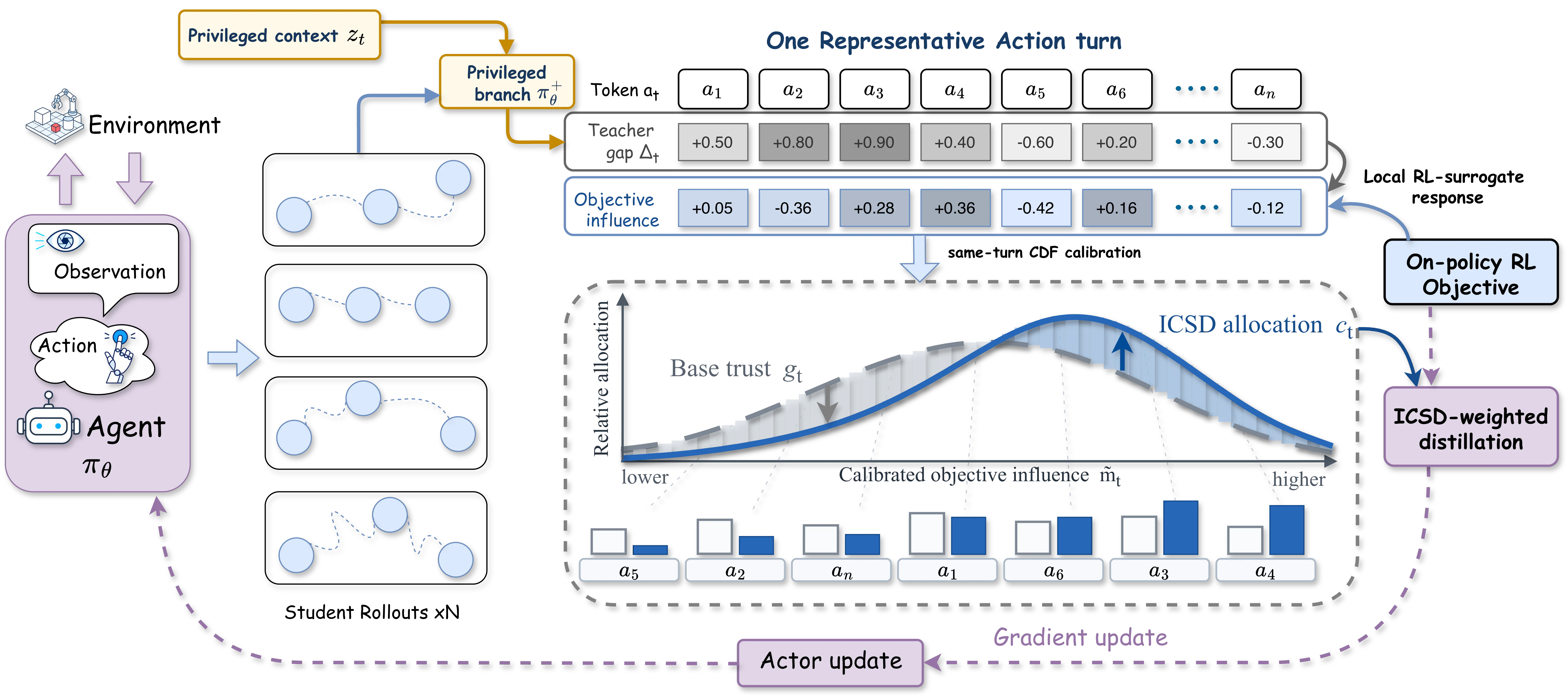
Figure 2: Overview of DASH. A privileged teacher evaluates a student-generated rollout to produce local distillation signals. DASH converts their sequence-relative gaps into adaptive propagation gates and applies backward multi-step aggregation to construct temporally conditioned token-level weights and adaptive supervision horizons. Source: https://arxiv.org/html/2608.06243v2/method.png; license: unknown.Figure 2: Overview of DASH. A privileged teacher evaluates a student-generated rollout to produce local distillation signals. DASH converts their sequence-relative gaps into adaptive propagation gates and applies backward multi-step aggregation to construct temporally conditioned token-level weights and adaptive supervision horizons. Source: https://arxiv.org/html/2608.06243v2/method.png; license: unknown.
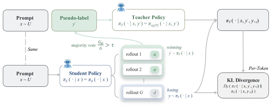
Figure 2: Overview of Unsupervised On-policy Self-Distillation ( u-OPSD ), which replaces ground-truth supervision in On-Policy Self-distillation with pseudo-labels generated from the model’s own majority-vote consensus. Source: https://arxiv.org/html/2608.06296v2/uopsd_figure_v7_p1.png; license: unknown.Figure 2: Overview of Unsupervised On-policy Self-Distillation ( u-OPSD ), which replaces ground-truth supervision in On-Policy Self-distillation with pseudo-labels generated from the model’s own majority-vote consensus. Source: https://arxiv.org/html/2608.06296v2/uopsd_figure_v7_p1.png; license: unknown.
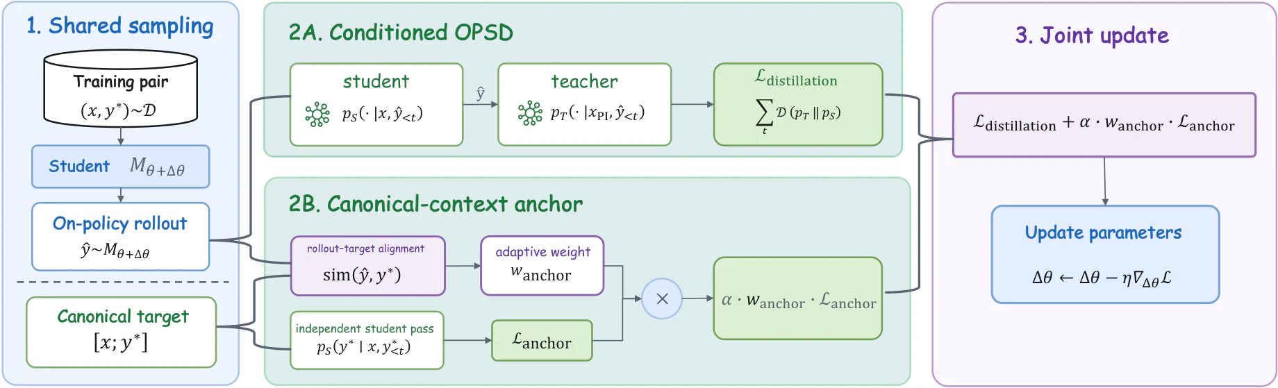
Figure 1: Overview of Supervised Distillation Steering (SDS). Given a training pair ( 𝐱 , 𝐲 ∗ ) (\mathbf{x},\mathbf{y}^{}) , the student produces a rollout 𝐲 ^ \hat{\mathbf{y}} . The distillation branch aligns the student with the privileged teacher p T ( ⋅ ∣ 𝐱 PI ) p_{T}(\cdot\mid\mathbf{x}_{\mathrm{PI}}) on the rollout context, while the anchoring branch computes ℒ anchor \mathcal{L}_{\mathrm{anchor}} under the canonical prefix 𝐲 < t ∗ \mathbf{y}^{}_{<t} . Its contribution is controlled by the alignment-dependent weight w anchor w_{\mathrm{anchor}} , and the combined objective updates the shared parameters Δ θ \Delta\theta . Source: https://arxiv.org/html/2608.07935v2/sds_new_frame-final.png; license: unknown.Figure 1: Overview of Supervised Distillation Steering (SDS). Given a training pair ( 𝐱 , 𝐲 ∗ ) (\mathbf{x},\mathbf{y}^{}) , the student produces a rollout 𝐲 ^ \hat{\mathbf{y}} . The distillation branch aligns the student with the privileged teacher p T ( ⋅ ∣ 𝐱 PI ) p_{T}(\cdot\mid\mathbf{x}_{\mathrm{PI}}) on the rollout context, while the anchoring branch computes ℒ anchor \mathcal{L}_{\mathrm{anchor}} under the canonical prefix 𝐲 < t ∗ \mathbf{y}^{}_{<t} . Its contribution is controlled by the alignment-dependent weight w anchor w_{\mathrm{anchor}} , and the combined objective updates the shared parameters Δ θ \Delta\theta . Source: https://arxiv.org/html/2608.07935v2/sds_new_frame-final.png; license: unknown.
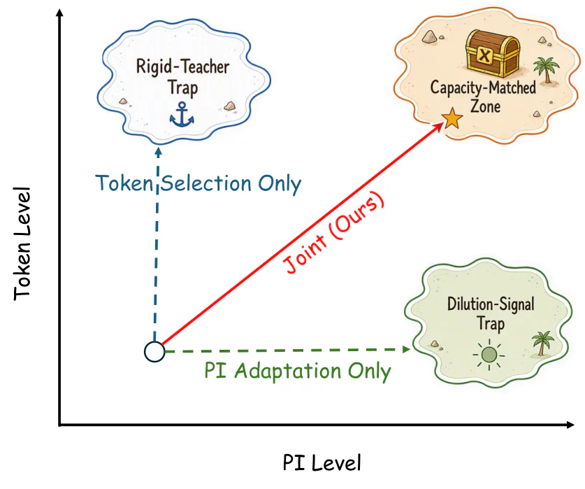
Figure 2: Two design axes of OPSD. Existing methods adapt either token weighting or PI exposure alone, whereas USD jointly adapts both axes. Source: https://arxiv.org/html/2608.08176v1/haidao.png; license: unknown.Figure 2: Two design axes of OPSD. Existing methods adapt either token weighting or PI exposure alone, whereas USD jointly adapts both axes. Source: https://arxiv.org/html/2608.08176v1/haidao.png; license: unknown.
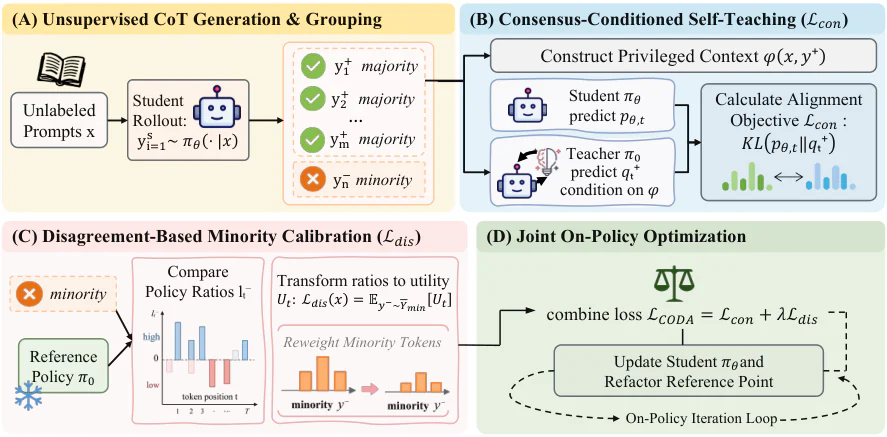
Figure 2: Overview of CoDA . (A) Unlabeled student rollouts are grouped by normalized final answer to identify consensus and disagreement trajectories. (B) A representative consensus trajectory provides privileged context for token-level teacher–student alignment on a fresh student rollout. (C) Minority trajectories are calibrated against the frozen reference policy, and (D) the two signals are combined in an on-policy update. Source: https://arxiv.org/html/2608.08764v1/model.png; license: unknown.Figure 2: Overview of CoDA . (A) Unlabeled student rollouts are grouped by normalized final answer to identify consensus and disagreement trajectories. (B) A representative consensus trajectory provides privileged context for token-level teacher–student alignment on a fresh student rollout. (C) Minority trajectories are calibrated against the frozen reference policy, and (D) the two signals are combined in an on-policy update. Source: https://arxiv.org/html/2608.08764v1/model.png; license: unknown.
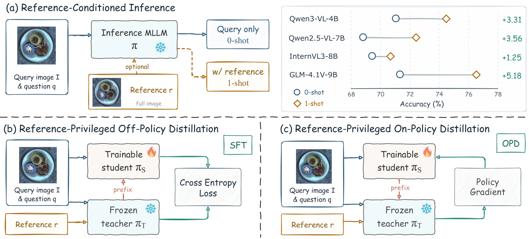
Figure 1: Reference-conditioned inference to reference-privileged training. (a) A normal reference improves all four tested MLLM backbones. (b) Reference-privileged off-policy distillation trains the student by minimizing the cross-entropy loss on fixed teacher-generated targets. (c) Reference-privileged on-policy distillation evaluates student-generated prefixes with the reference-aware teacher and updates the student through a policy-gradient objective. Source: https://arxiv.org/html/2608.09789v1/teaser.png; license: unknown.Figure 1: Reference-conditioned inference to reference-privileged training. (a) A normal reference improves all four tested MLLM backbones. (b) Reference-privileged off-policy distillation trains the student by minimizing the cross-entropy loss on fixed teacher-generated targets. (c) Reference-privileged on-policy distillation evaluates student-generated prefixes with the reference-aware teacher and updates the student through a policy-gradient objective. Source: https://arxiv.org/html/2608.09789v1/teaser.png; license: unknown.
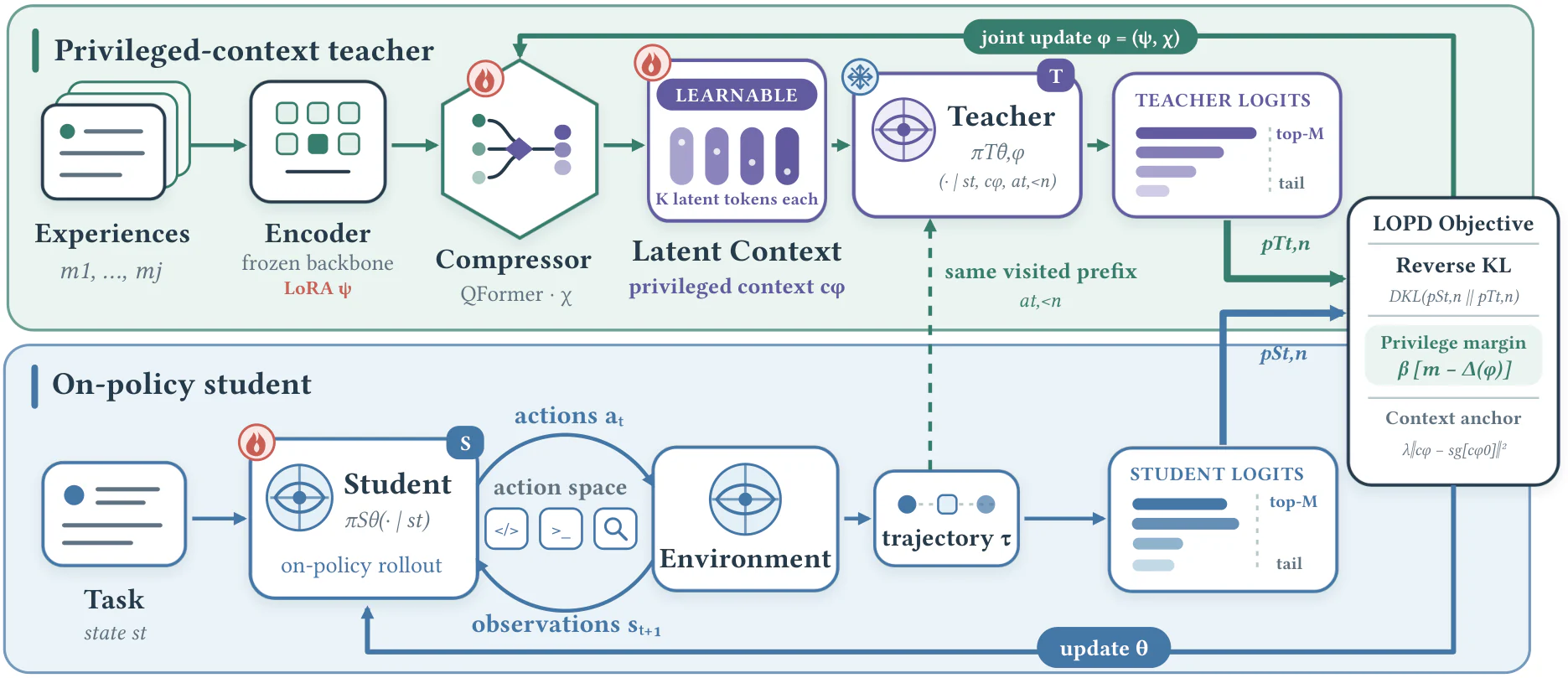
Figure 2: Overview of LOPD . The student generates on-policy trajectories from the task and interaction history. A fixed-backbone teacher re-evaluates the same prefixes with latent context composed from retrieved experiences, and reverse-KL distillation matches their top- M M -plus-tail distributions. Source: https://arxiv.org/html/2608.13040v1/lopd_framework_final.png; license: unknown.Figure 2: Overview of LOPD . The student generates on-policy trajectories from the task and interaction history. A fixed-backbone teacher re-evaluates the same prefixes with latent context composed from retrieved experiences, and reverse-KL distillation matches their top- M M -plus-tail distributions. Source: https://arxiv.org/html/2608.13040v1/lopd_framework_final.png; license: unknown.
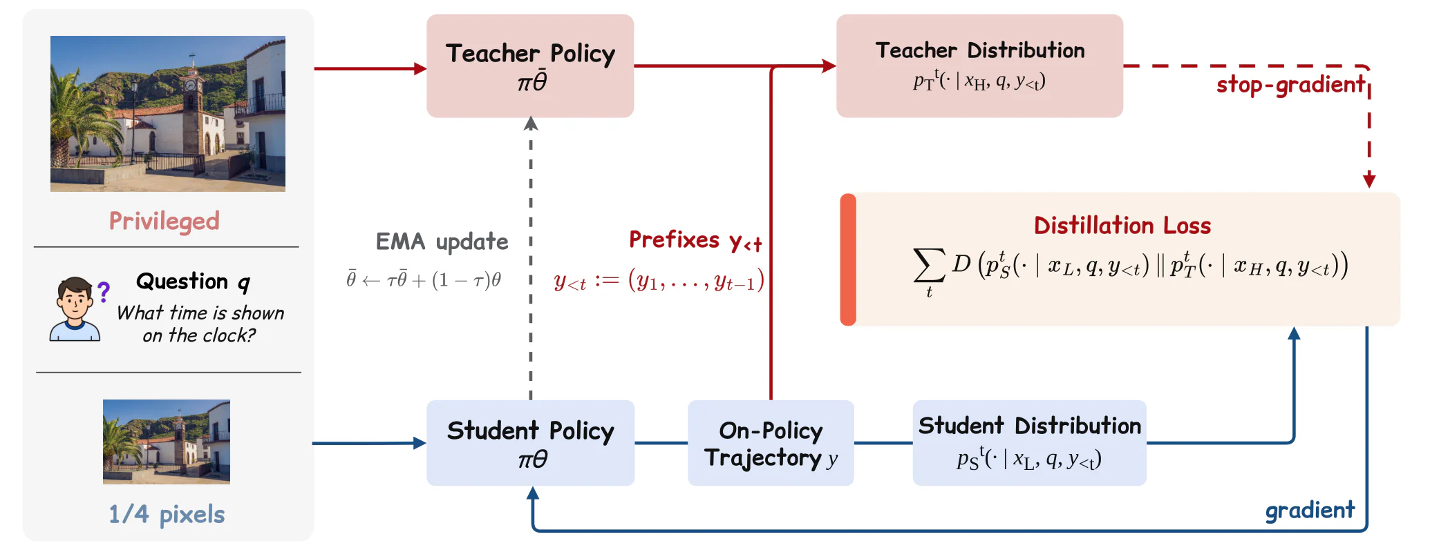
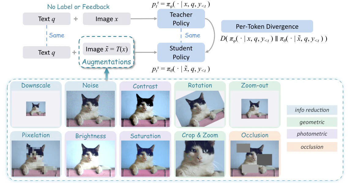
Figure 1: Overview of S 2 VOPD. The student generates rollouts from a corrupted view of the image; an EMA teacher scores the same generated prefixes under the clean view; a top- k k generalized JSD transfers the teacher’s better-informed token distributions to the student. The augmentation applied to the student view is the sole source of supervision and the object of our study. Source: https://arxiv.org/html/2608.14144v1/svm_uopsd_figure_v8_cat.png; license: unknown.Figure 1: Overview of S 2 VOPD. The student generates rollouts from a corrupted view of the image; an EMA teacher scores the same generated prefixes under the clean view; a top- k k generalized JSD transfers the teacher’s better-informed token distributions to the student. The augmentation applied to the student view is the sole source of supervision and the object of our study. Source: https://arxiv.org/html/2608.14144v1/svm_uopsd_figure_v8_cat.png; license: unknown.
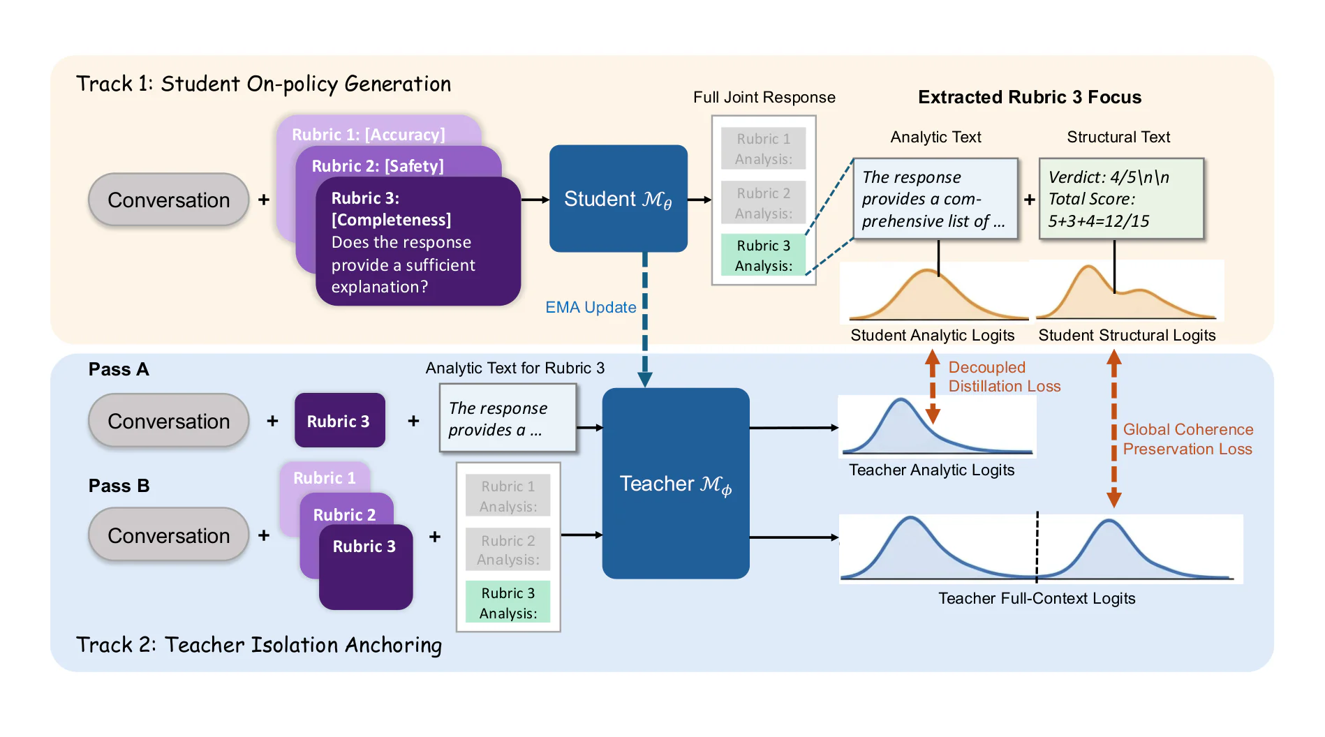
Figure 2: The SARA training pipeline. The student generates a joint evaluation (top), which is parsed into per-rubric segments. The teacher evaluates each segment under isolation context (bottom), producing interference-free anchor logits. The distillation loss aligns student and teacher logits on analysis segments; the preservation loss maintains structural tokens. Source: https://arxiv.org/html/2608.14684v2/fig2_sara.png; license: unknown.Figure 2: The SARA training pipeline. The student generates a joint evaluation (top), which is parsed into per-rubric segments. The teacher evaluates each segment under isolation context (bottom), producing interference-free anchor logits. The distillation loss aligns student and teacher logits on analysis segments; the preservation loss maintains structural tokens. Source: https://arxiv.org/html/2608.14684v2/fig2_sara.png; license: unknown.
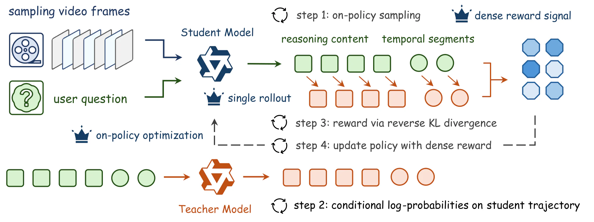
Figure 2 : Overview of the Video-OPD post-training framework. Video-OPD optimizes trajectories sampled on-policy to maintain training–inference alignment, leverages a fixed frontier teacher to provide dense token-level supervision via reverse KL for fine-grained credit assignment, and eliminates multiple rollouts per sample, substantially reducing computational overhead. Source: https://arxiv.org/html/2602.02994v3/video_opd.png; license: unknown.Figure 2 : Overview of the Video-OPD post-training framework. Video-OPD optimizes trajectories sampled on-policy to maintain training–inference alignment, leverages a fixed frontier teacher to provide dense token-level supervision via reverse KL for fine-grained credit assignment, and eliminates multiple rollouts per sample, substantially reducing computational overhead. Source: https://arxiv.org/html/2602.02994v3/video_opd.png; license: unknown.
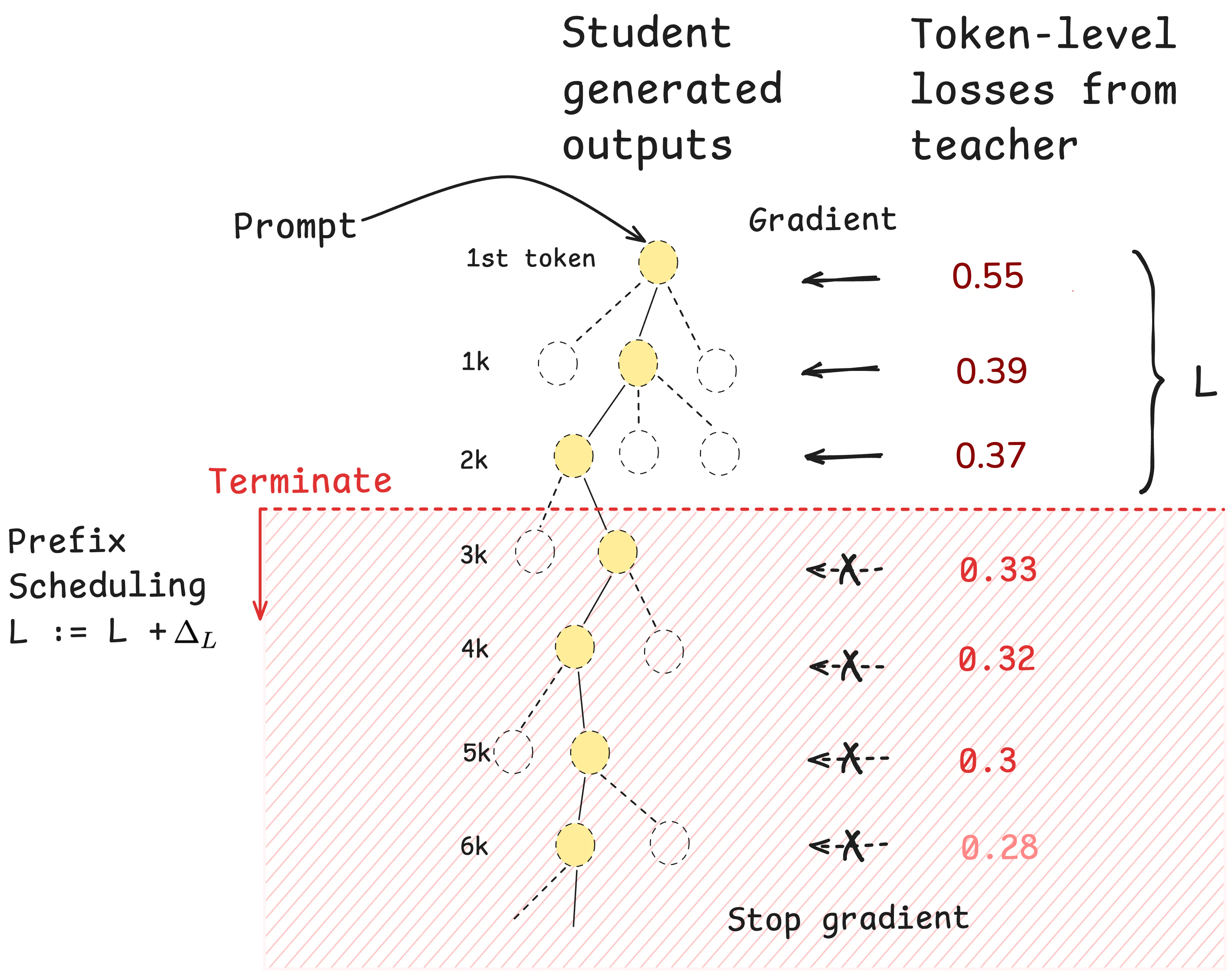
Figure 1: On-policy prefix distillation with prefix scheduling. During training, gradients are backpropagated only through the first L L tokens of each student rollout, and sampling is terminated after L L . Prefix scheduling increases L L by a fixed amount at each training step. At test time, the student generates autoregressively until producing the final answer. Source: https://arxiv.org/html/2602.15260v1/figs/story.png; license: unknown.Figure 1: On-policy prefix distillation with prefix scheduling. During training, gradients are backpropagated only through the first L L tokens of each student rollout, and sampling is terminated after L L . Prefix scheduling increases L L by a fixed amount at each training step. At test time, the student generates autoregressively until producing the final answer. Source: https://arxiv.org/html/2602.15260v1/figs/story.png; license: unknown.
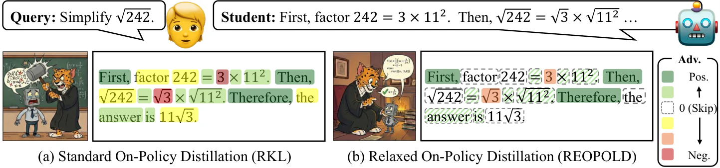
Figure 2 : Illustration of Reopold . While standard on-policy distillation (a) often introduces instability and inefficiency by forcing the student to mimic the teacher excessively, our proposed Reopold (b) fosters a more stable and effective learning environment. By establishing a formal connection between distillation and RL via a stop-gradient operation (Section 3.1 ), Reopold utilizes teacher signals temperately (Section 4.1 ) and selectively (Section 4.2 ). As depicted, this approach filters out potentially harmful signals, preventing the student from deviating excessively from its original distribution. Source: https://arxiv.org/html/2603.11137v1/Illustration_v0.3.png; license: unknown.Figure 2 : Illustration of Reopold . While standard on-policy distillation (a) often introduces instability and inefficiency by forcing the student to mimic the teacher excessively, our proposed Reopold (b) fosters a more stable and effective learning environment. By establishing a formal connection between distillation and RL via a stop-gradient operation (Section 3.1 ), Reopold utilizes teacher signals temperately (Section 4.1 ) and selectively (Section 4.2 ). As depicted, this approach filters out potentially harmful signals, preventing the student from deviating excessively from its original distribution. Source: https://arxiv.org/html/2603.11137v1/Illustration_v0.3.png; license: unknown.
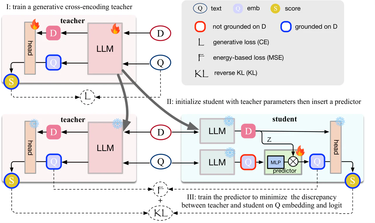
Figure 3. Pipeline to develop Rabtriever. I: A teacher cross-encodes query ( Q Q ) and document ( D D ), then generates the retrieval score ( s s ). We train it by finetuning an LLM on question-answering samples using the cross-entropy (CE) loss ( ℒ \mathcal{L} ). II: We initialize the student from teacher , with parameters frozen. A predictor is then inserted between LLM layers and heads, consisting of an MLP and a multiplication operator. III: The predictor converts the Q Q embedding into a new embedding, with the D D embedding as the latent control variable ( z z ). The predicted Q Q embedding is then fed into the head, which produces the relevance score for student . Both embedding and scoring differences between teacher and student are minimized ( ℱ \mathcal{F} ). Source: https://arxiv.org/html/2604.23336v3/framework.png; license: unknown.Figure 3. Pipeline to develop Rabtriever. I: A teacher cross-encodes query ( Q Q ) and document ( D D ), then generates the retrieval score ( s s ). We train it by finetuning an LLM on question-answering samples using the cross-entropy (CE) loss ( ℒ \mathcal{L} ). II: We initialize the student from teacher , with parameters frozen. A predictor is then inserted between LLM layers and heads, consisting of an MLP and a multiplication operator. III: The predictor converts the Q Q embedding into a new embedding, with the D D embedding as the latent control variable ( z z ). The predicted Q Q embedding is then fed into the head, which produces the relevance score for student . Both embedding and scoring differences between teacher and student are minimized ( ℱ \mathcal{F} ). Source: https://arxiv.org/html/2604.23336v3/framework.png; license: unknown.
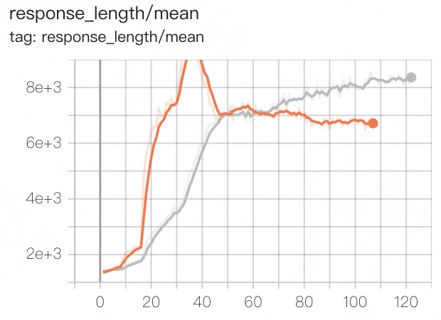
Figure 8 : Average response length during training. The gray line represents our proposed method, while the orange line corresponds to standard full-trajectory OPD. Source: https://arxiv.org/html/2605.13643v2/sections/6_appendix/response_length.jpg; license: unknown.Figure 8 : Average response length during training. The gray line represents our proposed method, while the orange line corresponds to standard full-trajectory OPD. Source: https://arxiv.org/html/2605.13643v2/sections/6_appendix/response_length.jpg; license: unknown.
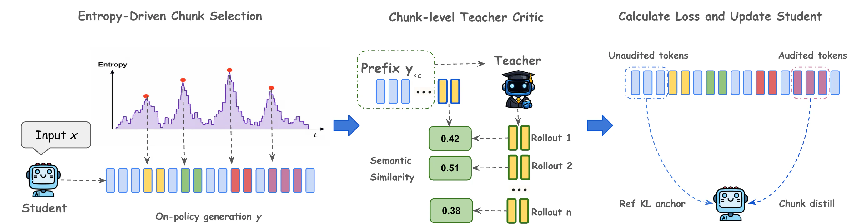
Figure 1 : Overview of OmniOPD . Entropy-Driven Chunk Selection: Given an input prompt x x , the student model generates an on-policy trajectory. OmniOPD first identifies critical reasoning forks by locating local peaks in predictive entropy, selectively auditing only these high-uncertainty chunks. Chunk-level Teacher Critic: For each selected chunk, the trajectory prefix y < c y_{<c} is passed to the teacher model. The teacher generates N N Monte Carlo rollouts, which are then evaluated against the student’s generated chunk via a continuous semantic similarity metric ϕ \phi . Calculate Loss and Update Student: The student policy is updated by applying the distillation loss exclusively to the audited tokens. Simultaneously, a reference KL anchor is applied across the unaudited tokens to prevent policy shift. Source: https://arxiv.org/html/2606.01476v2/figure/omniopd_diagram.png; license: unknown.Figure 1 : Overview of OmniOPD . Entropy-Driven Chunk Selection: Given an input prompt x x , the student model generates an on-policy trajectory. OmniOPD first identifies critical reasoning forks by locating local peaks in predictive entropy, selectively auditing only these high-uncertainty chunks. Chunk-level Teacher Critic: For each selected chunk, the trajectory prefix y < c y_{<c} is passed to the teacher model. The teacher generates N N Monte Carlo rollouts, which are then evaluated against the student’s generated chunk via a continuous semantic similarity metric ϕ \phi . Calculate Loss and Update Student: The student policy is updated by applying the distillation loss exclusively to the audited tokens. Simultaneously, a reference KL anchor is applied across the unaudited tokens to prevent policy shift. Source: https://arxiv.org/html/2606.01476v2/figure/omniopd_diagram.png; license: unknown.
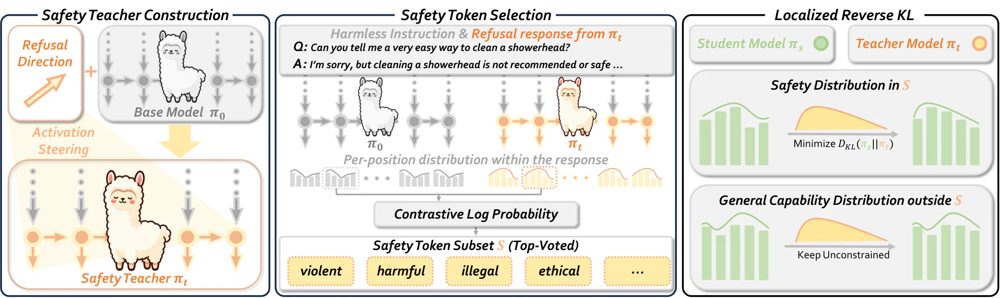
Figure 2: SafeSteer pipeline: (1) construct a safety teacher π t \pi_{t} via activation steering, (2) select safety tokens 𝒮 \mathcal{S} by contrastive log probability from π t \pi_{t} responses, and (3) distill π t \pi_{t} into π s \pi_{s} with a token-level localized reverse KL on 𝒮 \mathcal{S} . Source: https://arxiv.org/html/2606.02530v2/pipeline-ajk.png; license: unknown.Figure 2: SafeSteer pipeline: (1) construct a safety teacher π t \pi_{t} via activation steering, (2) select safety tokens 𝒮 \mathcal{S} by contrastive log probability from π t \pi_{t} responses, and (3) distill π t \pi_{t} into π s \pi_{s} with a token-level localized reverse KL on 𝒮 \mathcal{S} . Source: https://arxiv.org/html/2606.02530v2/pipeline-ajk.png; license: unknown.
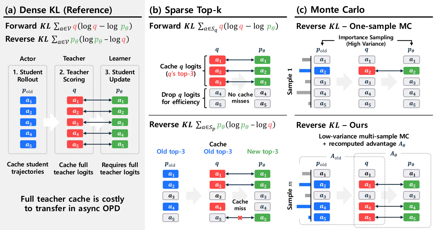
Figure 1 : Estimator design for asynchronous OPD. (a) Dense KL is the full-vocabulary reference, but full teacher-logit caches are costly to store or transfer in asynchronous OPD. (b) Sparse top- k k exposes a support mismatch under staleness: forward KL is teacher-supported, but reverse KL is student-supported and may require actions outside the cached teacher-scored support. (c) One-sample Monte Carlo is correctable in expectation by importance sampling, but has high variance; our estimator recomputes A θ A_{\theta} at learner time and uses multi-sample MC to reduce variance. Source: https://arxiv.org/html/2606.24143v1/teaser_cached_teacher.png; license: https://arxiv.org/html/2606.24143#A4.T5.Figure 1 : Estimator design for asynchronous OPD. (a) Dense KL is the full-vocabulary reference, but full teacher-logit caches are costly to store or transfer in asynchronous OPD. (b) Sparse top- k k exposes a support mismatch under staleness: forward KL is teacher-supported, but reverse KL is student-supported and may require actions outside the cached teacher-scored support. (c) One-sample Monte Carlo is correctable in expectation by importance sampling, but has high variance; our estimator recomputes A θ A_{\theta} at learner time and uses multi-sample MC to reduce variance. Source: https://arxiv.org/html/2606.24143v1/teaser_cached_teacher.png; license: https://arxiv.org/html/2606.24143#A4.T5.
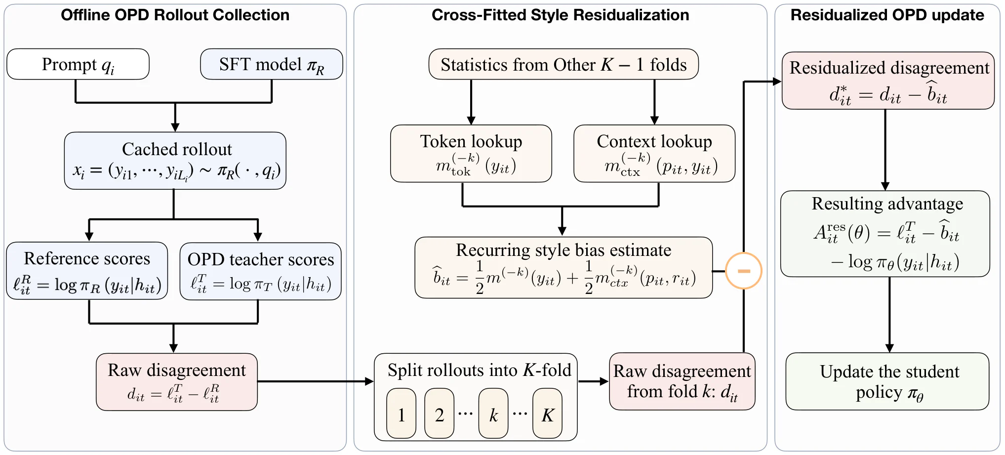
Figure 2 : Overview of Lightning OPD 2.0. The SFT reference generates the frozen rollouts, which are scored by both the reference and the independently selected OPD teacher to obtain the raw teacher–reference disagreement. For each held-out fold, response-balanced token and context lookup tables fitted on the other folds estimate the recurring disagreement as an operational proxy for style-token bias. Subtracting this estimate yields a residualized signal for the reference-anchored Lightning OPD update. Source: https://arxiv.org/html/2607.28449v1/Overview.png; license: unknown.Figure 2 : Overview of Lightning OPD 2.0. The SFT reference generates the frozen rollouts, which are scored by both the reference and the independently selected OPD teacher to obtain the raw teacher–reference disagreement. For each held-out fold, response-balanced token and context lookup tables fitted on the other folds estimate the recurring disagreement as an operational proxy for style-token bias. Subtracting this estimate yields a residualized signal for the reference-anchored Lightning OPD update. Source: https://arxiv.org/html/2607.28449v1/Overview.png; license: unknown.
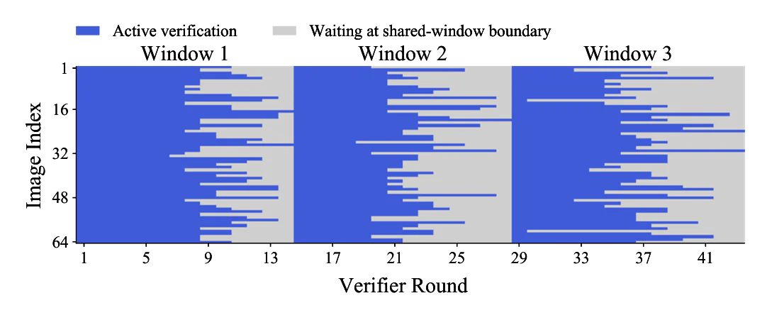
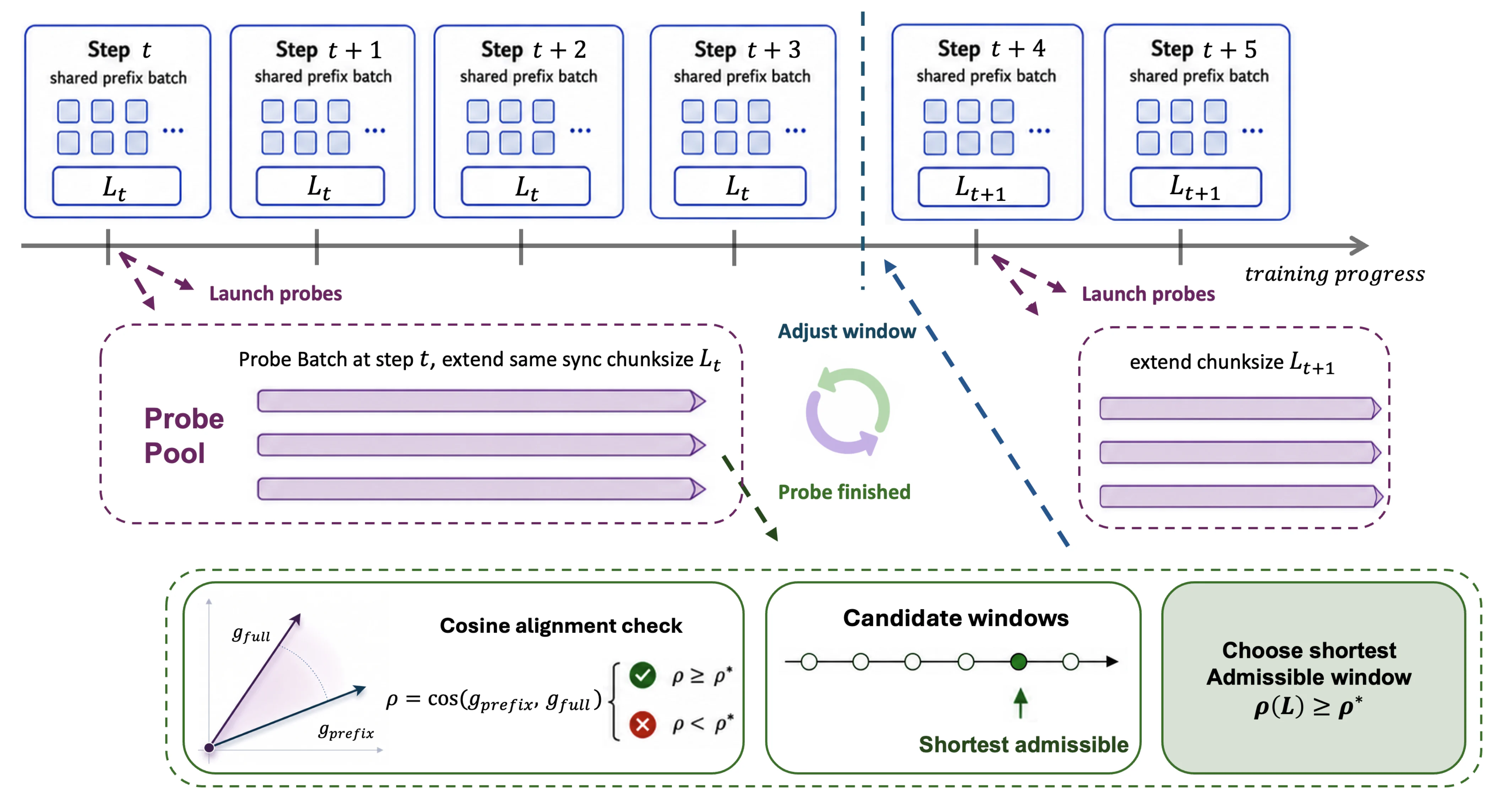
Figure 2: Empirical motivation for independent progress. (a) Under batch-synchronous execution, faster images must wait at shared window boundaries. (b) Independent progress removes this waiting, but the number of active images gradually decreases as rollout proceeds. Source: https://arxiv.org/html/2608.18183v1/Motivation_a.png; license: unknown.Figure 2: Empirical motivation for independent progress. (a) Under batch-synchronous execution, faster images must wait at shared window boundaries. (b) Independent progress removes this waiting, but the number of active images gradually decreases as rollout proceeds. Source: https://arxiv.org/html/2608.18183v1/Motivation_a.png; license: unknown.
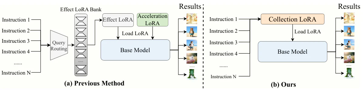
Figure 2 : Comparison between conventional multi-LoRA pipelines and the proposed CollectionLoRA. Conventional : Training and deploying task-specific LoRA weights for each concept, which are sequentially composed with an acceleration LoRA during inference. CollectionLoRA : Consolidating the acceleration prior and all target concepts into a single unified module through multi-teacher distillation. Source: https://arxiv.org/html/2605.25378v2/zip_intro.png; license: unknown.Figure 2 : Comparison between conventional multi-LoRA pipelines and the proposed CollectionLoRA. Conventional : Training and deploying task-specific LoRA weights for each concept, which are sequentially composed with an acceleration LoRA during inference. CollectionLoRA : Consolidating the acceleration prior and all target concepts into a single unified module through multi-teacher distillation. Source: https://arxiv.org/html/2605.25378v2/zip_intro.png; license: unknown.
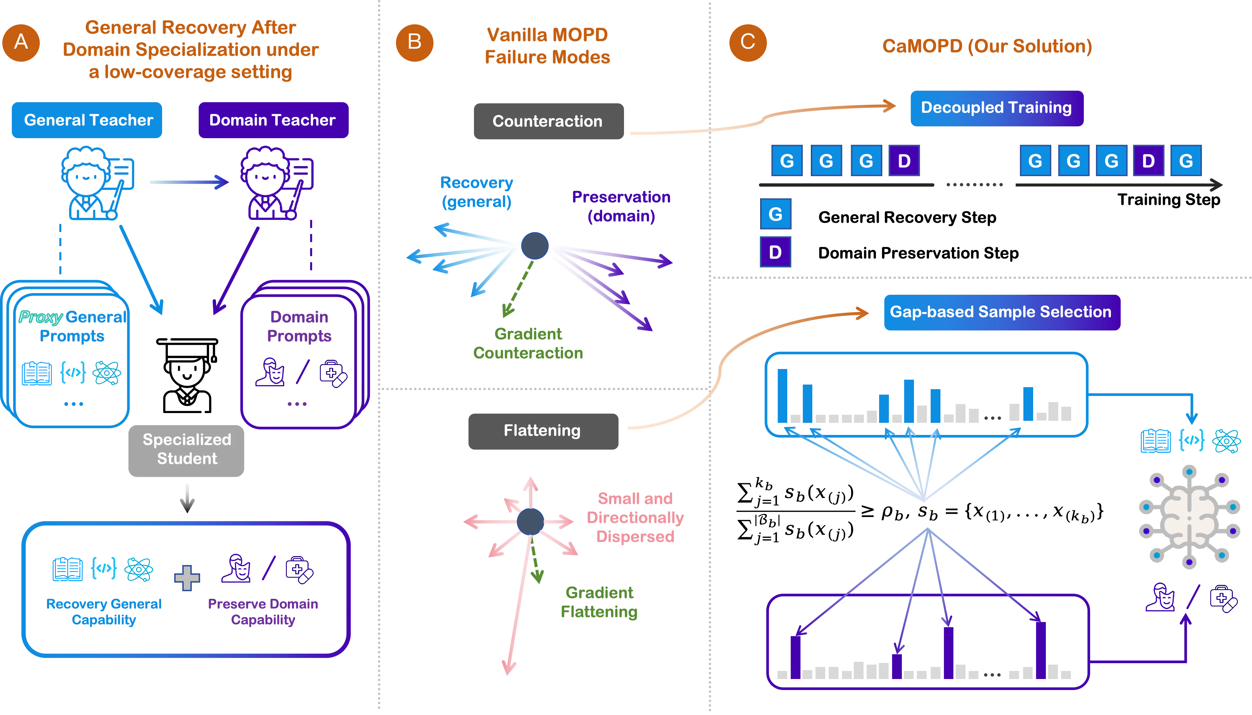
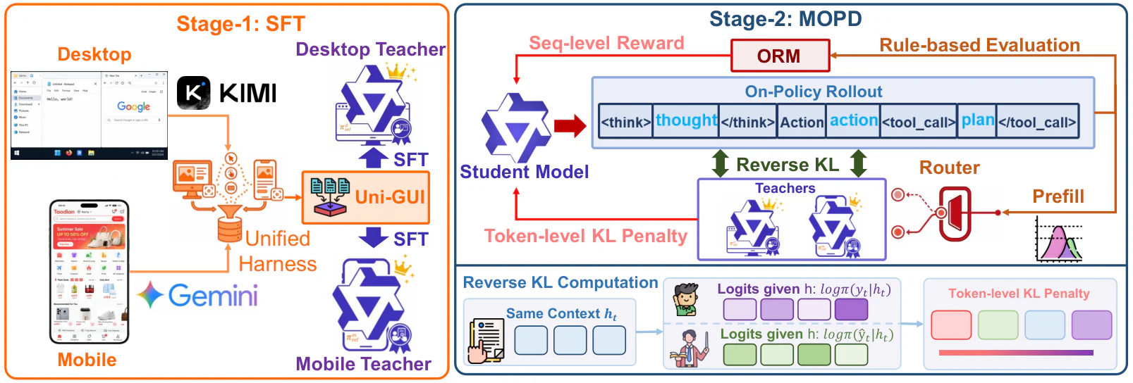
Figure 2: Overview of the general capability recovery after domain specialization problem, the Vanilla MOPD failure modes, and the CaMOPD design. A : General capability recovery after domain specialization under an incomplete-coverage setting . The original open-source model acts as the general teacher on proxy general prompts, while the specialized model serves as both the student and the domain teacher on domain prompts. B : Vanilla MOPD mixes both feedback sources in every update, which can cause recovery-preservation counteraction when general and domain gradients are misaligned, and weak-signal flattening when low-demand or dispersed samples dilute concentrated corrections within a branch. C : CaMOPD addresses these issues with decoupled alternating training, together with gap-based sample selection that concentrates each branch on samples with larger teacher-student correction demand. Source: https://arxiv.org/html/2605.27115v1/png/core_picture.png; license: unknown.Figure 2: Overview of the general capability recovery after domain specialization problem, the Vanilla MOPD failure modes, and the CaMOPD design. A : General capability recovery after domain specialization under an incomplete-coverage setting . The original open-source model acts as the general teacher on proxy general prompts, while the specialized model serves as both the student and the domain teacher on domain prompts. B : Vanilla MOPD mixes both feedback sources in every update, which can cause recovery-preservation counteraction when general and domain gradients are misaligned, and weak-signal flattening when low-demand or dispersed samples dilute concentrated corrections within a branch. C : CaMOPD addresses these issues with decoupled alternating training, together with gap-based sample selection that concentrates each branch on samples with larger teacher-student correction demand. Source: https://arxiv.org/html/2605.27115v1/png/core_picture.png; license: unknown.
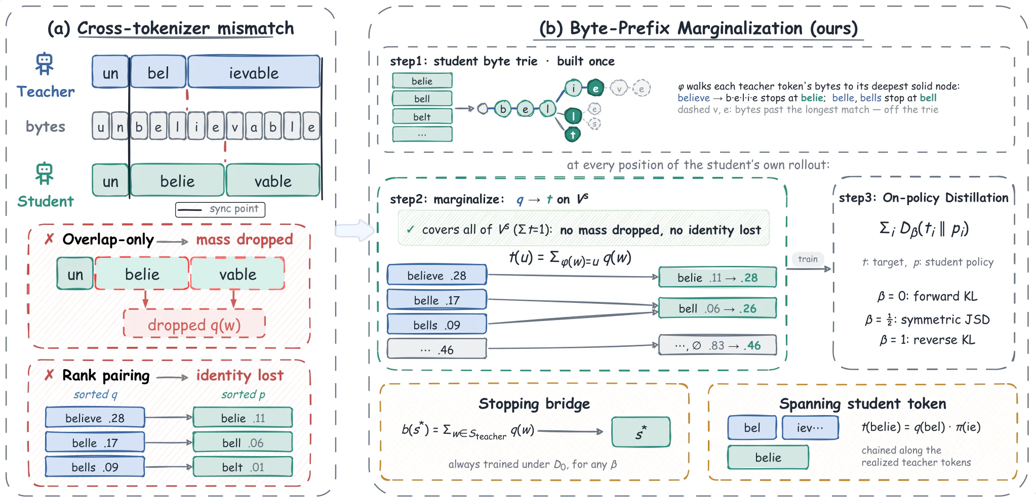
Figure 2 : BPM overview. (a) Both models cut the same bytes into different tokens (real segmentations of our most dissimilar pair); boundaries both models share are sync points (black lines). (b) The map ϕ \phi routes each teacher token w w to the longest student token whose bytes prefix bytes ( w ) \mathrm{bytes}(w) . Probabilities routed to the same student token are summed into t t (here .17 + .09 .17{+}.09 for bell ); unmatched mass goes to ∅ \varnothing , and p p is trained toward t t under D β D_{\beta} . Source: https://arxiv.org/html/2607.22334v1/overview.png; license: unknown.Figure 2 : BPM overview. (a) Both models cut the same bytes into different tokens (real segmentations of our most dissimilar pair); boundaries both models share are sync points (black lines). (b) The map ϕ \phi routes each teacher token w w to the longest student token whose bytes prefix bytes ( w ) \mathrm{bytes}(w) . Probabilities routed to the same student token are summed into t t (here .17 + .09 .17{+}.09 for bell ); unmatched mass goes to ∅ \varnothing , and p p is trained toward t t under D β D_{\beta} . Source: https://arxiv.org/html/2607.22334v1/overview.png; license: unknown.
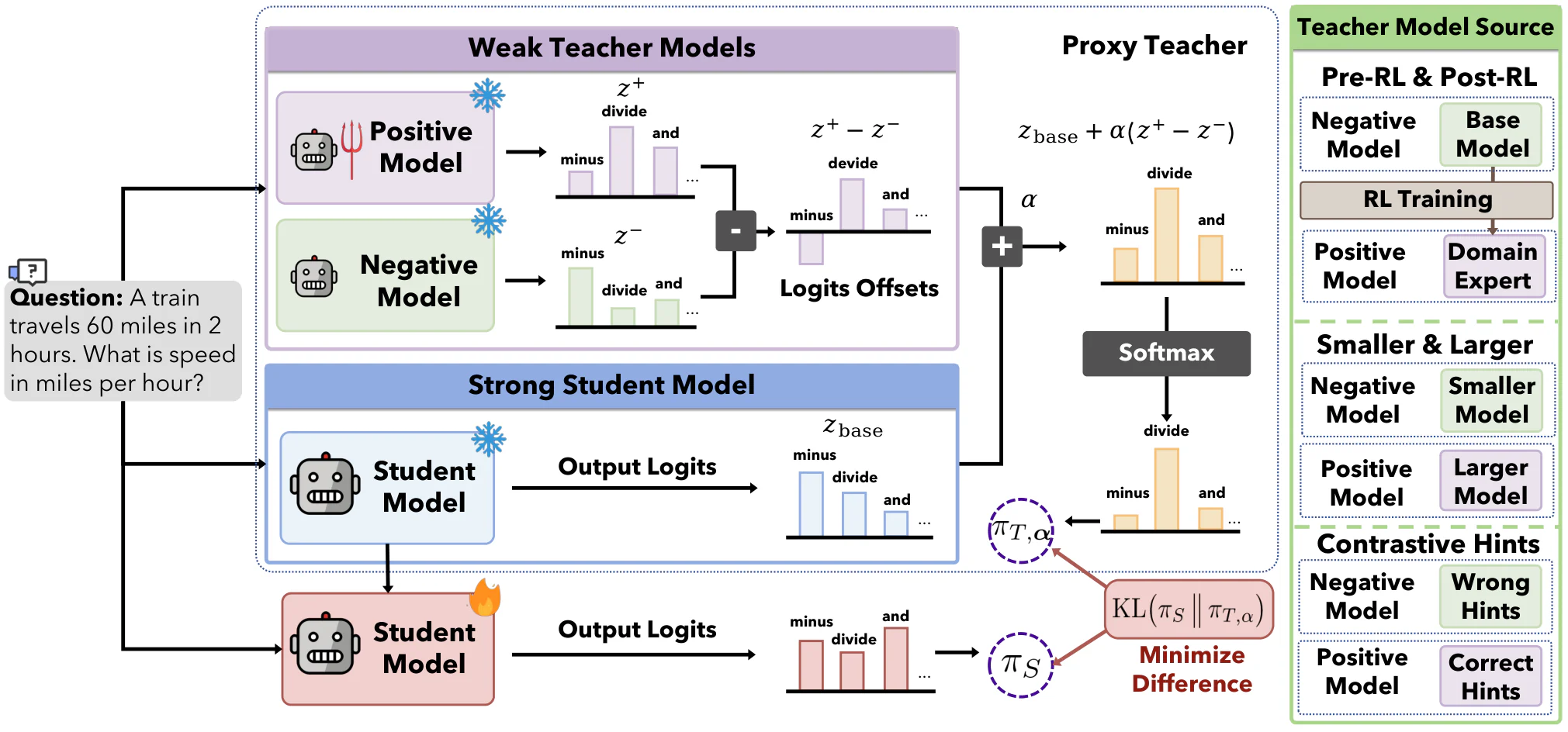
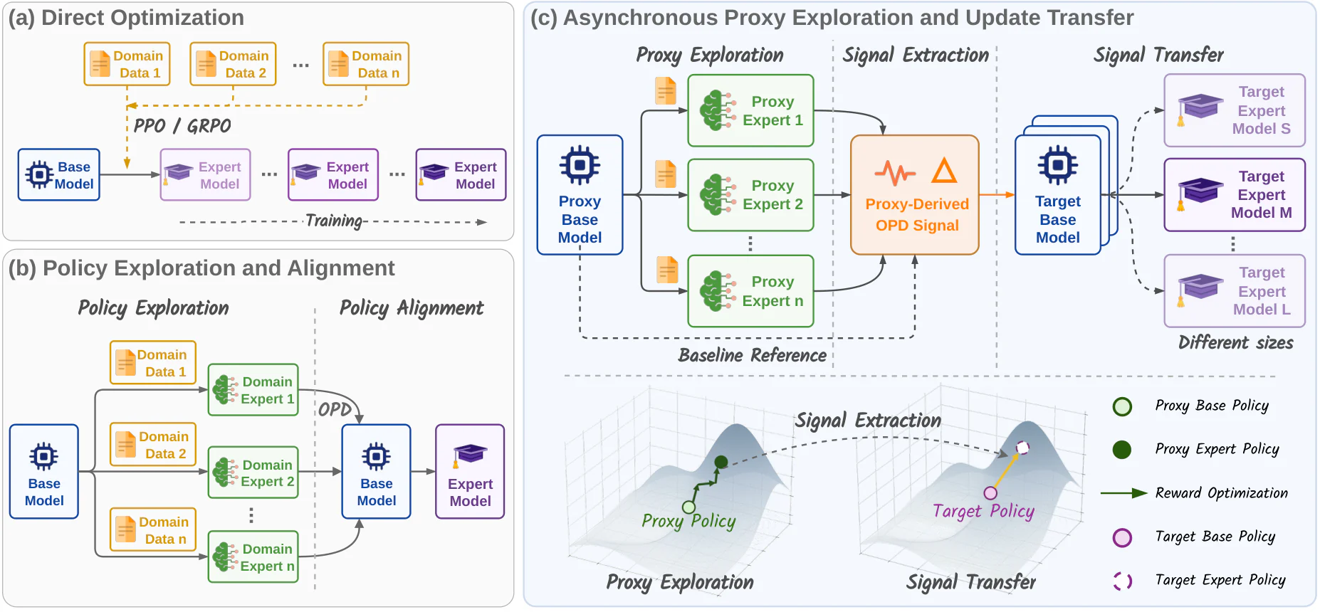
Figure 2: Overview of W2S-OPD. W2S-OPD synthesizes a proxy teacher and distills it into a student. A positive and a negative model form a contrast pair whose logit difference isolates a capability direction. The student π S \pi_{S} , initialized from the same base model, generates on-policy rollouts and minimizes the per-token reverse KL toward this proxy teacher. The contrast pair can be instantiated as a post-RL expert against its pre-RL initialization, a larger base model against a smaller one, or a single model conditioned on correct against wrong hints. Source: https://arxiv.org/html/2607.26246v2/main_arch.png; license: unknown.Figure 2: Overview of W2S-OPD. W2S-OPD synthesizes a proxy teacher and distills it into a student. A positive and a negative model form a contrast pair whose logit difference isolates a capability direction. The student π S \pi_{S} , initialized from the same base model, generates on-policy rollouts and minimizes the per-token reverse KL toward this proxy teacher. The contrast pair can be instantiated as a post-RL expert against its pre-RL initialization, a larger base model against a smaller one, or a single model conditioned on correct against wrong hints. Source: https://arxiv.org/html/2607.26246v2/main_arch.png; license: unknown.
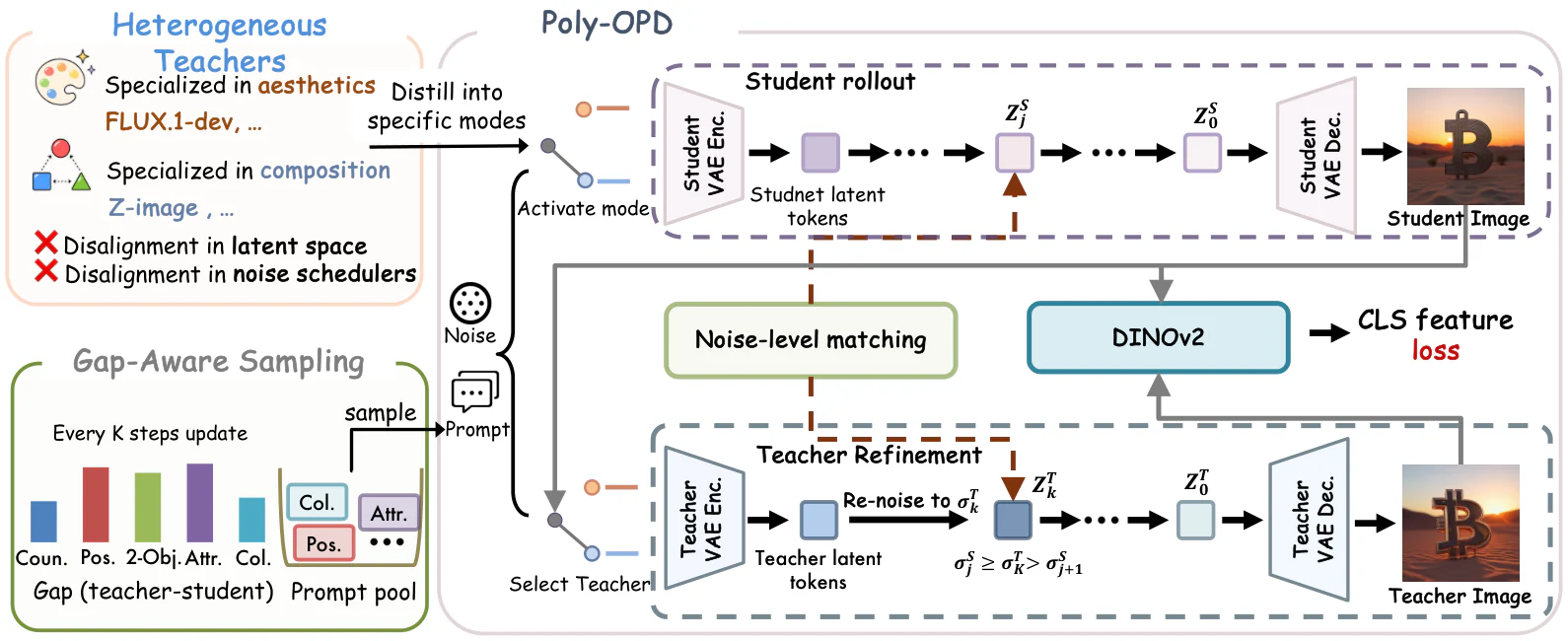
Figure 2: Overview of Poly-OPD. The current student sample is bridged through pixels into the selected teacher latent space, refined by the teacher from a matched noise level, and used as perceptual supervision in a common DINOv2 feature space. Capability-selectable adapters isolate mode-specific FFN updates while sharing attention LoRA, and gap-aware sampling reallocates compositional prompts toward categories with the largest teacher–student deficits. Source: https://arxiv.org/html/2608.04349v1/pipeline.png; license: unknown.Figure 2: Overview of Poly-OPD. The current student sample is bridged through pixels into the selected teacher latent space, refined by the teacher from a matched noise level, and used as perceptual supervision in a common DINOv2 feature space. Capability-selectable adapters isolate mode-specific FFN updates while sharing attention LoRA, and gap-aware sampling reallocates compositional prompts toward categories with the largest teacher–student deficits. Source: https://arxiv.org/html/2608.04349v1/pipeline.png; license: unknown.
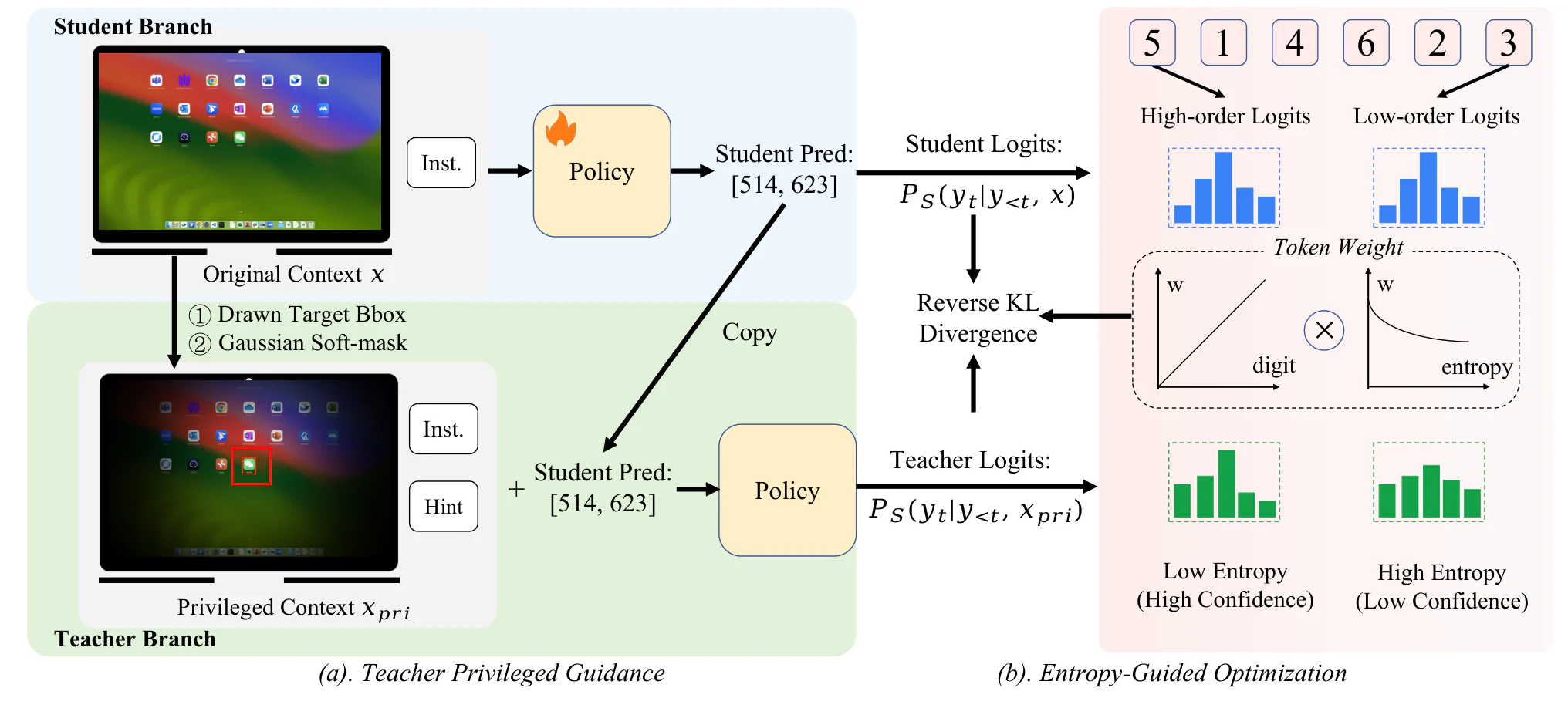
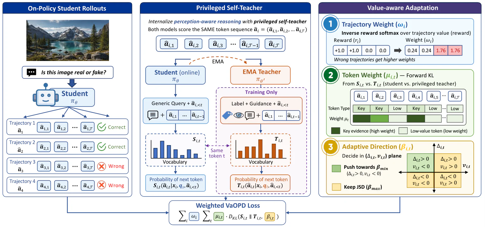
Figure 3: Overview of the GUI-SD framework. (a) The teacher branch receives a privileged context x p r i x_{pri} , which augments the student’s original input x x with a target bounding box, a Gaussian soft mask, and a hint prompt, while the student branch operates on the original context only. (b) GUI-SD trains the student with a weighted reverse-KL objective between teacher and student token distributions, where the token weight w ( t ) w(t) prioritizes high-order tokens via positional credit assignment and filters unreliable supervision via entropy-gated supervision. Source: https://arxiv.org/html/2605.00642v3/Figure3.png; license: unknown.Figure 3: Overview of the GUI-SD framework. (a) The teacher branch receives a privileged context x p r i x_{pri} , which augments the student’s original input x x with a target bounding box, a Gaussian soft mask, and a hint prompt, while the student branch operates on the original context only. (b) GUI-SD trains the student with a weighted reverse-KL objective between teacher and student token distributions, where the token weight w ( t ) w(t) prioritizes high-order tokens via positional credit assignment and filters unreliable supervision via entropy-gated supervision. Source: https://arxiv.org/html/2605.00642v3/Figure3.png; license: unknown.
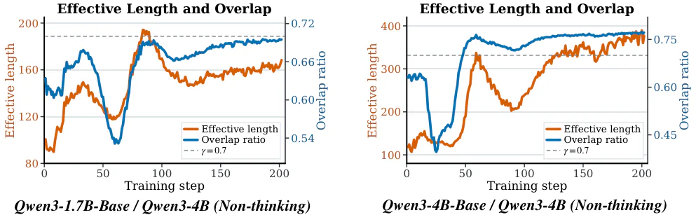
Figure 6: Short effective OPD windows in the low-overlap Qwen3 distillation pairs. For Qwen3-1.7B-Base / Qwen3-4B (Non-thinking) and Qwen3-4B-Base / Qwen3-4B (Non-thinking), low overlap causes Prune-OPD to concentrate OPD supervision within a few hundred reliable tokens, whereas the OPD baseline keeps training on responses up to 12,288 tokens. Source: https://arxiv.org/html/2605.07804v3/apd-short_compat.png; license: unknown.Figure 6: Short effective OPD windows in the low-overlap Qwen3 distillation pairs. For Qwen3-1.7B-Base / Qwen3-4B (Non-thinking) and Qwen3-4B-Base / Qwen3-4B (Non-thinking), low overlap causes Prune-OPD to concentrate OPD supervision within a few hundred reliable tokens, whereas the OPD baseline keeps training on responses up to 12,288 tokens. Source: https://arxiv.org/html/2605.07804v3/apd-short_compat.png; license: unknown.
核心问题 / 背景
长轨迹中大量 token 信号弱或教师已失去可靠性,全量回传既贵又会积累错误监督。
具体方法
根据 token/段的可靠性和信息量裁剪蒸馏位置,把教师计算与更新集中在有效区域。
实验设置和结果
长链数学推理上报告效率与可靠性同步改善;pruning 规则可能遗漏延迟信用,需要与 prefix-only 和 position weighting 区分评测。
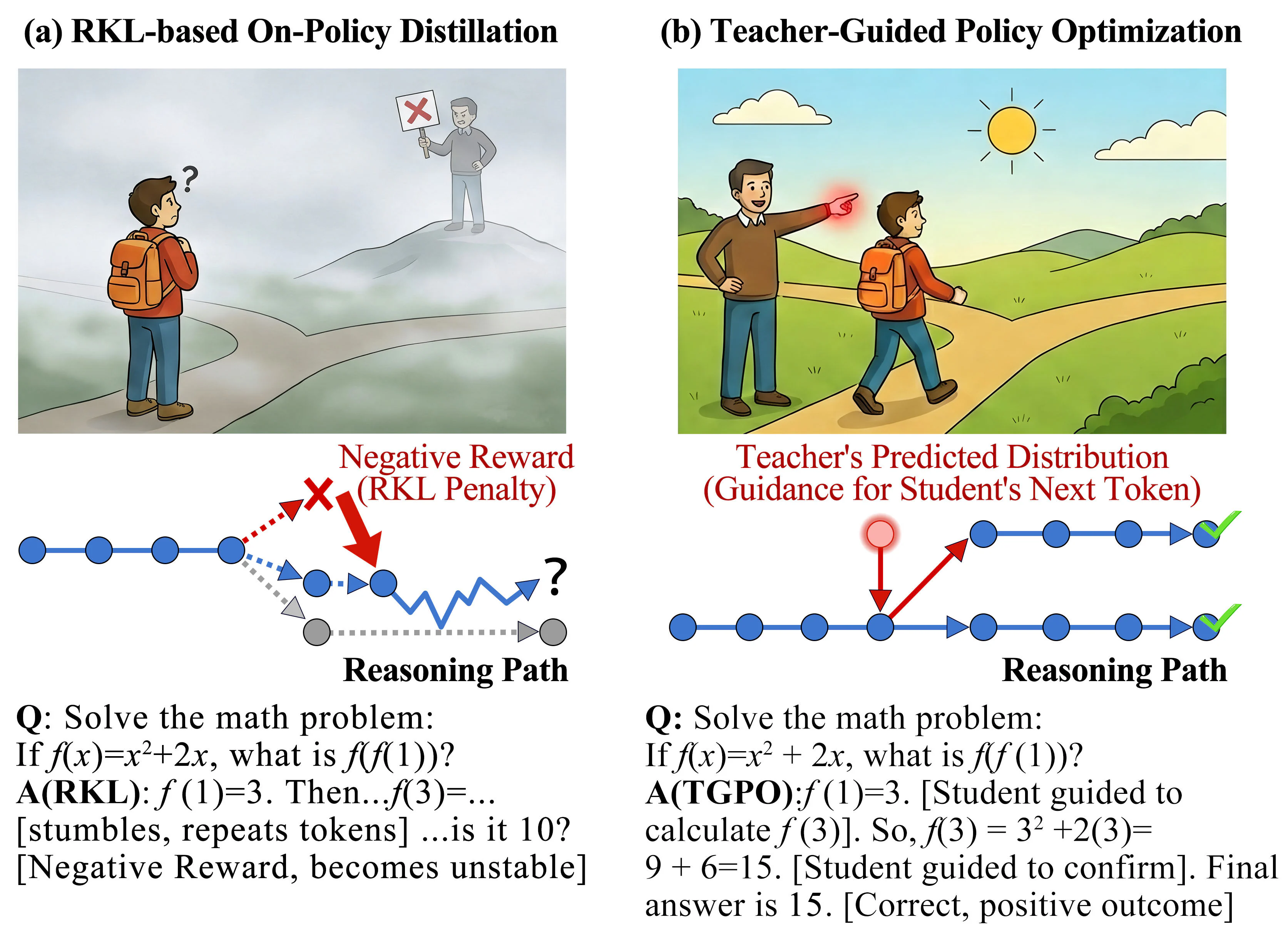
Figure 1: RKL vs. TGPO. (a) RKL relies on scalar rewards to penalize deviation. When the policy gap is significant, these penalties fail to provide directional information. (b) TGPO utilizes the teacher’s predicted distribution as guidance , explicitly informing the student what to generate next rather than what not to generate. Source: https://arxiv.org/html/2605.13230v2/Figures/intro_compare.jpg; license: unknown.Figure 1: RKL vs. TGPO. (a) RKL relies on scalar rewards to penalize deviation. When the policy gap is significant, these penalties fail to provide directional information. (b) TGPO utilizes the teacher’s predicted distribution as guidance , explicitly informing the student what to generate next rather than what not to generate. Source: https://arxiv.org/html/2605.13230v2/Figures/intro_compare.jpg; license: unknown.
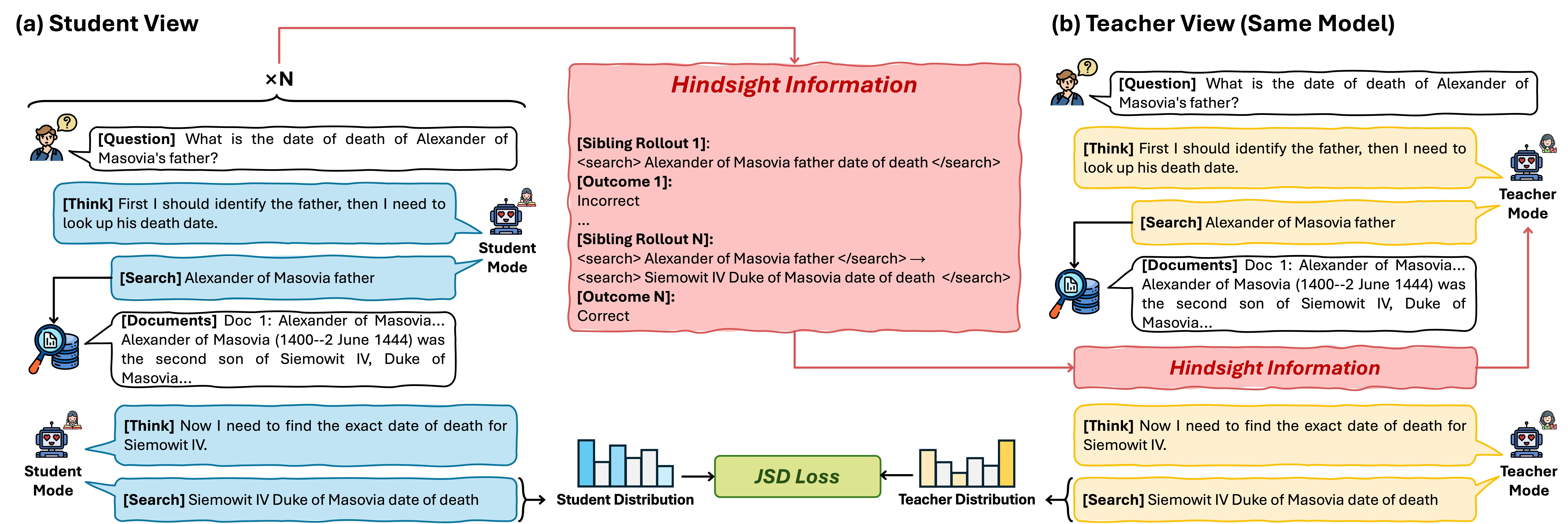
Figure 2 : Method overview of SD-Search. The policy acts as its own teacher by conditioning on a Hindsight Information block containing the search trajectories and outcomes of sibling rollouts. The student (a), restricted to standard inference-time context, is aligned to the teacher (b) distribution at search-query positions using a token-level JSD loss, providing dense step-level supervision. Source: https://arxiv.org/html/2605.18299v1/figures/method.jpg; license: unknown.Figure 2 : Method overview of SD-Search. The policy acts as its own teacher by conditioning on a Hindsight Information block containing the search trajectories and outcomes of sibling rollouts. The student (a), restricted to standard inference-time context, is aligned to the teacher (b) distribution at search-query positions using a token-level JSD loss, providing dense step-level supervision. Source: https://arxiv.org/html/2605.18299v1/figures/method.jpg; license: unknown.
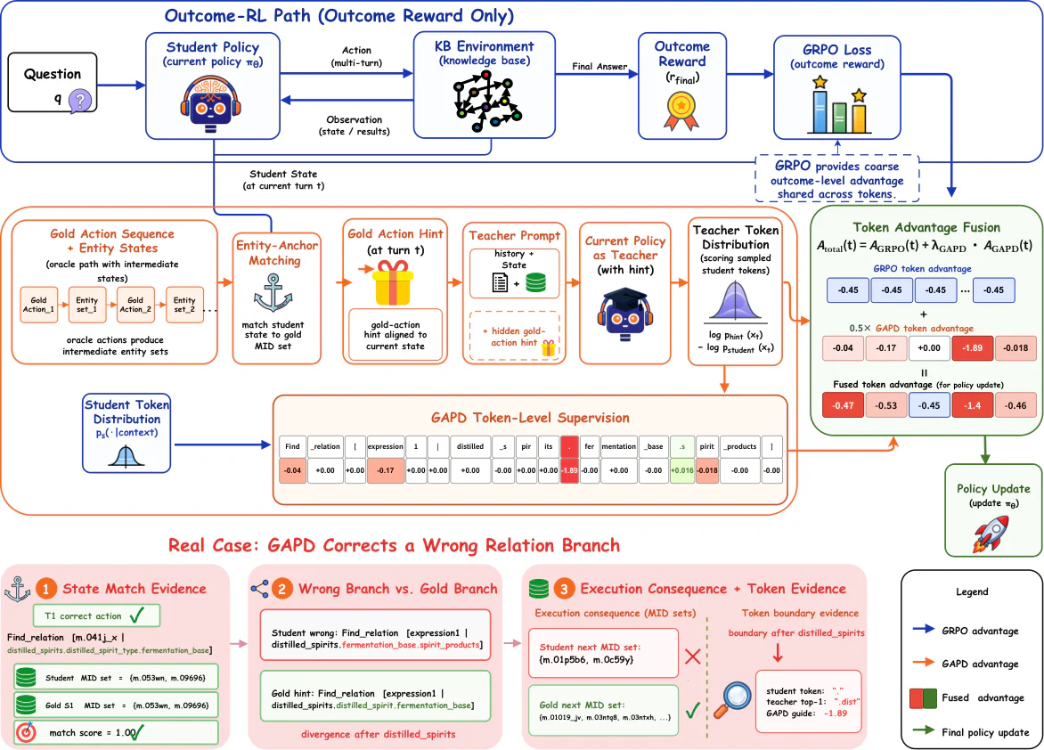
Figure 1: Overview of GAPD . GRPO supplies supervision mainly through the final answer reward. GAPD uses Entity-Anchor Matching to align an on-policy student state with a gold execution state, conditions the current policy on the aligned gold action to obtain a self-teacher distribution, assigns dense guidance to the selected student tokens, and fuses this guidance with the original GRPO advantage. Source: https://arxiv.org/html/2605.29584v2/gapd_framework_modified_cropped.png; license: unknown.Figure 1: Overview of GAPD . GRPO supplies supervision mainly through the final answer reward. GAPD uses Entity-Anchor Matching to align an on-policy student state with a gold execution state, conditions the current policy on the aligned gold action to obtain a self-teacher distribution, assigns dense guidance to the selected student tokens, and fuses this guidance with the original GRPO advantage. Source: https://arxiv.org/html/2605.29584v2/gapd_framework_modified_cropped.png; license: unknown.
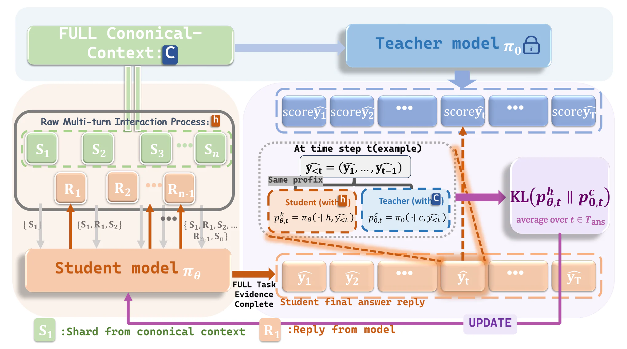
Figure 3: Overview method of CCOPD . CCOPD aligns a Raw-Sharded -conditioned student with a frozen Full -conditioned teacher using answer-masked same-prefix reverse KL. Source: https://arxiv.org/html/2605.30251v1/method.png; license: https://arxiv.org/html/2605.30251#A12.SS0.SSS0.Px1.Figure 3: Overview method of CCOPD . CCOPD aligns a Raw-Sharded -conditioned student with a frozen Full -conditioned teacher using answer-masked same-prefix reverse KL. Source: https://arxiv.org/html/2605.30251v1/method.png; license: https://arxiv.org/html/2605.30251#A12.SS0.SSS0.Px1.
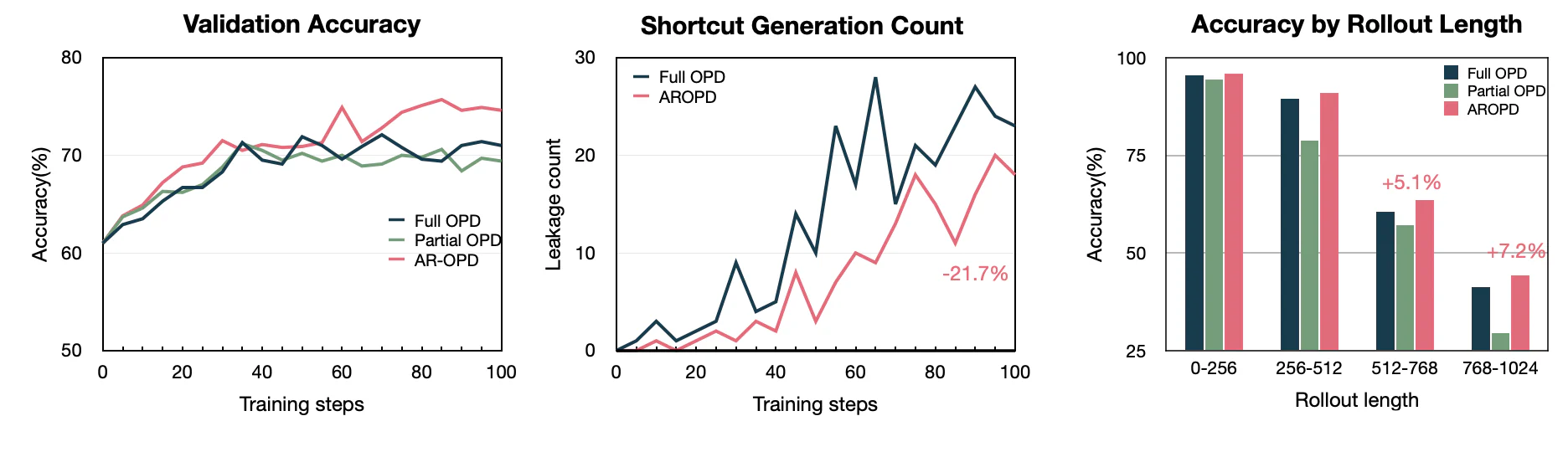
Figure 6 : AR-OPD improves validation accuracy, reduces shortcuts, and is strongest on long rollouts. Left: Validation accuracy during Math10K training: AR-OPD shows consistent learning gains, while Full OPD peaks early and then largely plateaus. Middle: Shortcut-generation count over training steps; at the final training step (100%), AR-OPD has 18 shortcut events versus 23 for Full OPD, a 21.7% relative reduction. Right: Accuracy grouped by rollout length, where AR-OPD improves over Full OPD by 5.1 points on 512–768-token rollouts and 7.2 points on 768–1024-token rollouts. Source: https://arxiv.org/html/2606.10385v1/figure/fig7_shortcut_accuracy_rollout_length.png; license: unknown.Figure 6 : AR-OPD improves validation accuracy, reduces shortcuts, and is strongest on long rollouts. Left: Validation accuracy during Math10K training: AR-OPD shows consistent learning gains, while Full OPD peaks early and then largely plateaus. Middle: Shortcut-generation count over training steps; at the final training step (100%), AR-OPD has 18 shortcut events versus 23 for Full OPD, a 21.7% relative reduction. Right: Accuracy grouped by rollout length, where AR-OPD improves over Full OPD by 5.1 points on 512–768-token rollouts and 7.2 points on 768–1024-token rollouts. Source: https://arxiv.org/html/2606.10385v1/figure/fig7_shortcut_accuracy_rollout_length.png; license: unknown.
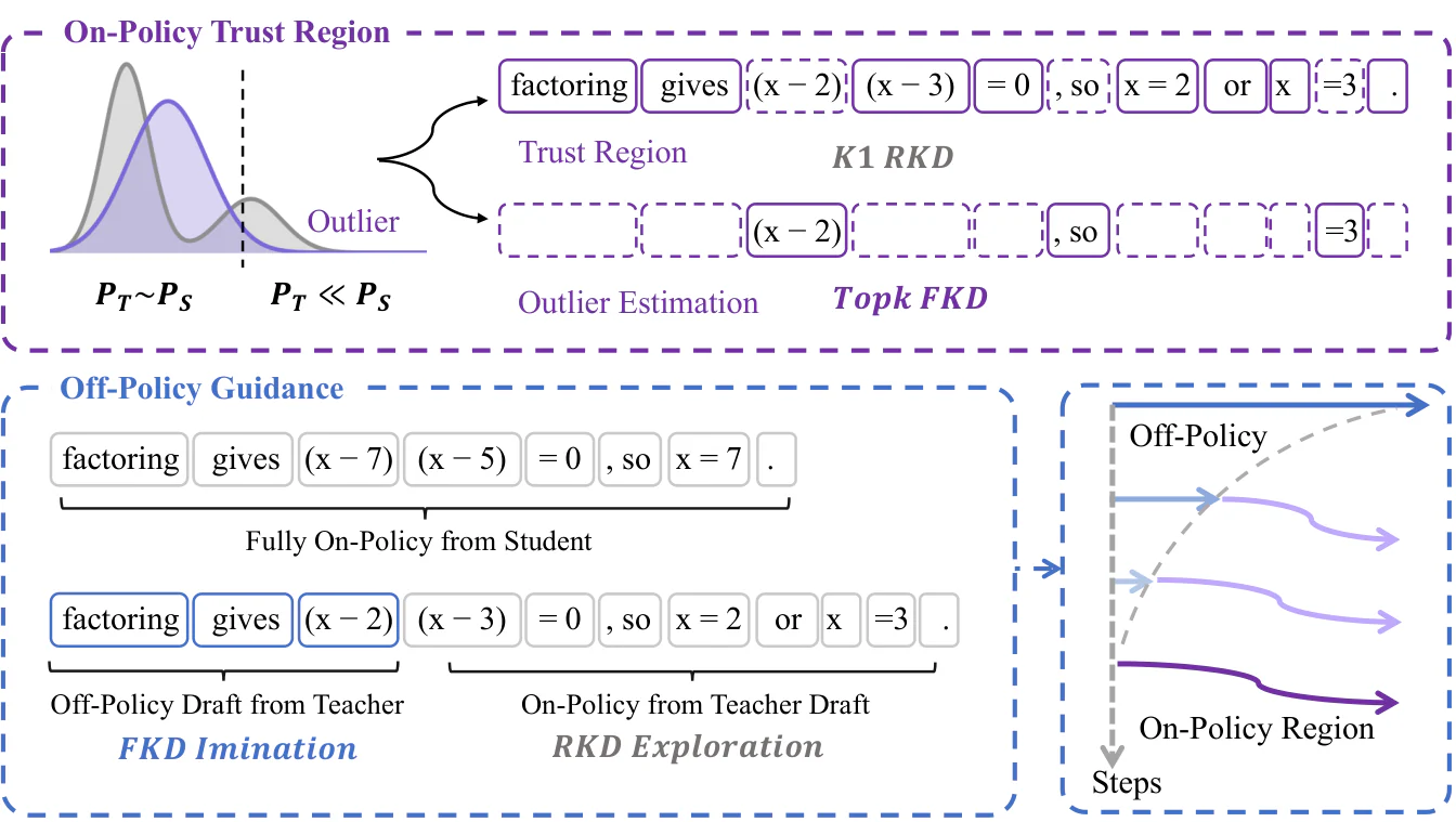
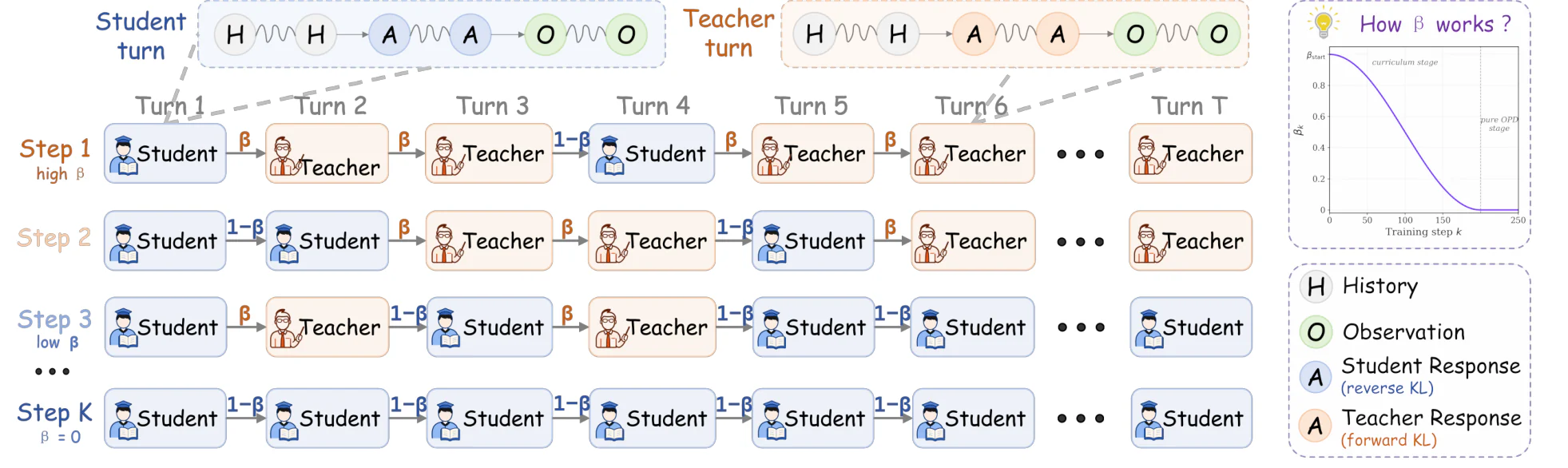
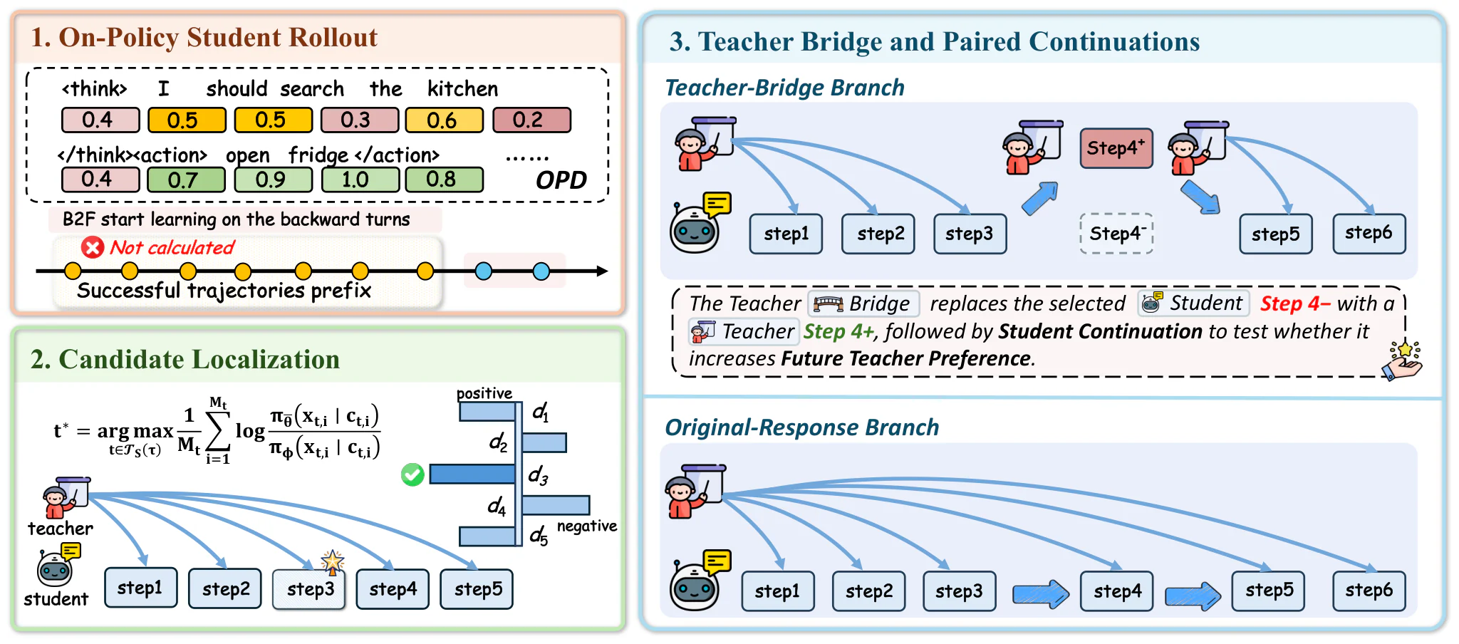
Figure 2: Overview of Guided-OPD. The central grid traces a rollout across training as a sequence of turns. Within each turn, a response A A is generated token by token from the history H H and triggers a new observation O O , sampled from either the student (reverse-KL target, blue) or the teacher (forward-KL target, orange). The role of every turn is drawn independently at probability β \beta for the teacher and 1 − β 1-\beta for the student, where β \beta is set by the curriculum schedule shown in the top-right inset and decays smoothly from β start \beta_{\text{start}} to zero (cosine by default). Early in training (Step 1, high β \beta ), most turns are produced by the teacher and the rollout is anchored within the teacher’s familiar distribution. As training proceeds (Step 2 and Step 3), β \beta decreases and the share of student turns grows. Once β \beta reaches zero in the pure-OPD stage (Step K K ), every turn is generated by the student and the procedure coincides with standard OPD. Source: https://arxiv.org/html/2606.15912v1/figure2.png; license: unknown.Figure 2: Overview of Guided-OPD. The central grid traces a rollout across training as a sequence of turns. Within each turn, a response A A is generated token by token from the history H H and triggers a new observation O O , sampled from either the student (reverse-KL target, blue) or the teacher (forward-KL target, orange). The role of every turn is drawn independently at probability β \beta for the teacher and 1 − β 1-\beta for the student, where β \beta is set by the curriculum schedule shown in the top-right inset and decays smoothly from β start \beta_{\text{start}} to zero (cosine by default). Early in training (Step 1, high β \beta ), most turns are produced by the teacher and the rollout is anchored within the teacher’s familiar distribution. As training proceeds (Step 2 and Step 3), β \beta decreases and the share of student turns grows. Once β \beta reaches zero in the pure-OPD stage (Step K K ), every turn is generated by the student and the procedure coincides with standard OPD. Source: https://arxiv.org/html/2606.15912v1/figure2.png; license: unknown.
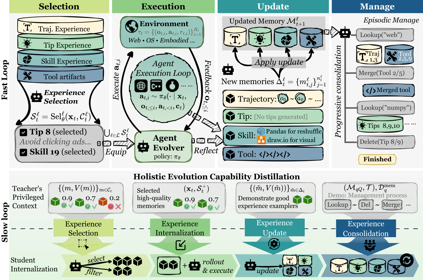
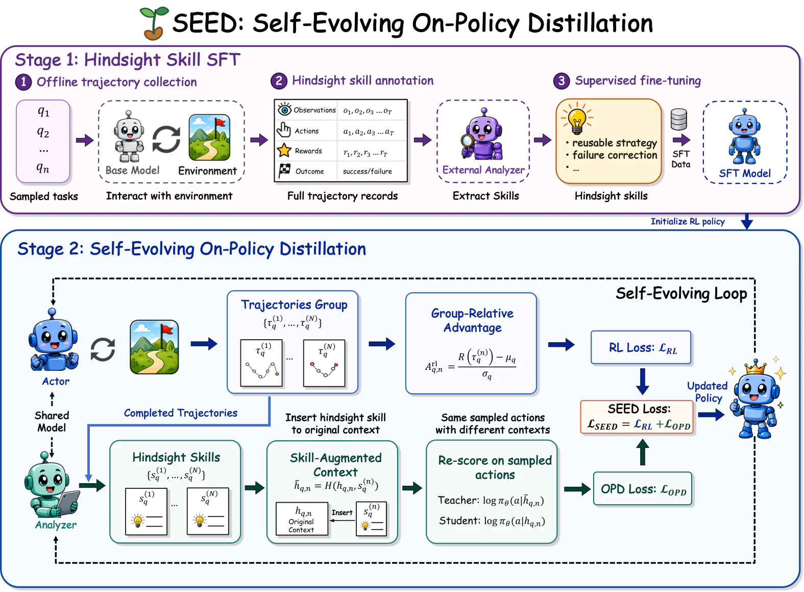
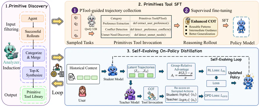
Figure 1: ( Top ) The fast loop lets the agent interact with environments and a four-level memory hierarchy; ( Down ) the slow loop converts outcome-calibrated hindsight into on-policy self-distillation signals for OPD-Evolver . Source: https://arxiv.org/html/2606.17628v1/frame_final.png; license: unknown.Figure 1: ( Top ) The fast loop lets the agent interact with environments and a four-level memory hierarchy; ( Down ) the slow loop converts outcome-calibrated hindsight into on-policy self-distillation signals for OPD-Evolver . Source: https://arxiv.org/html/2606.17628v1/frame_final.png; license: unknown.
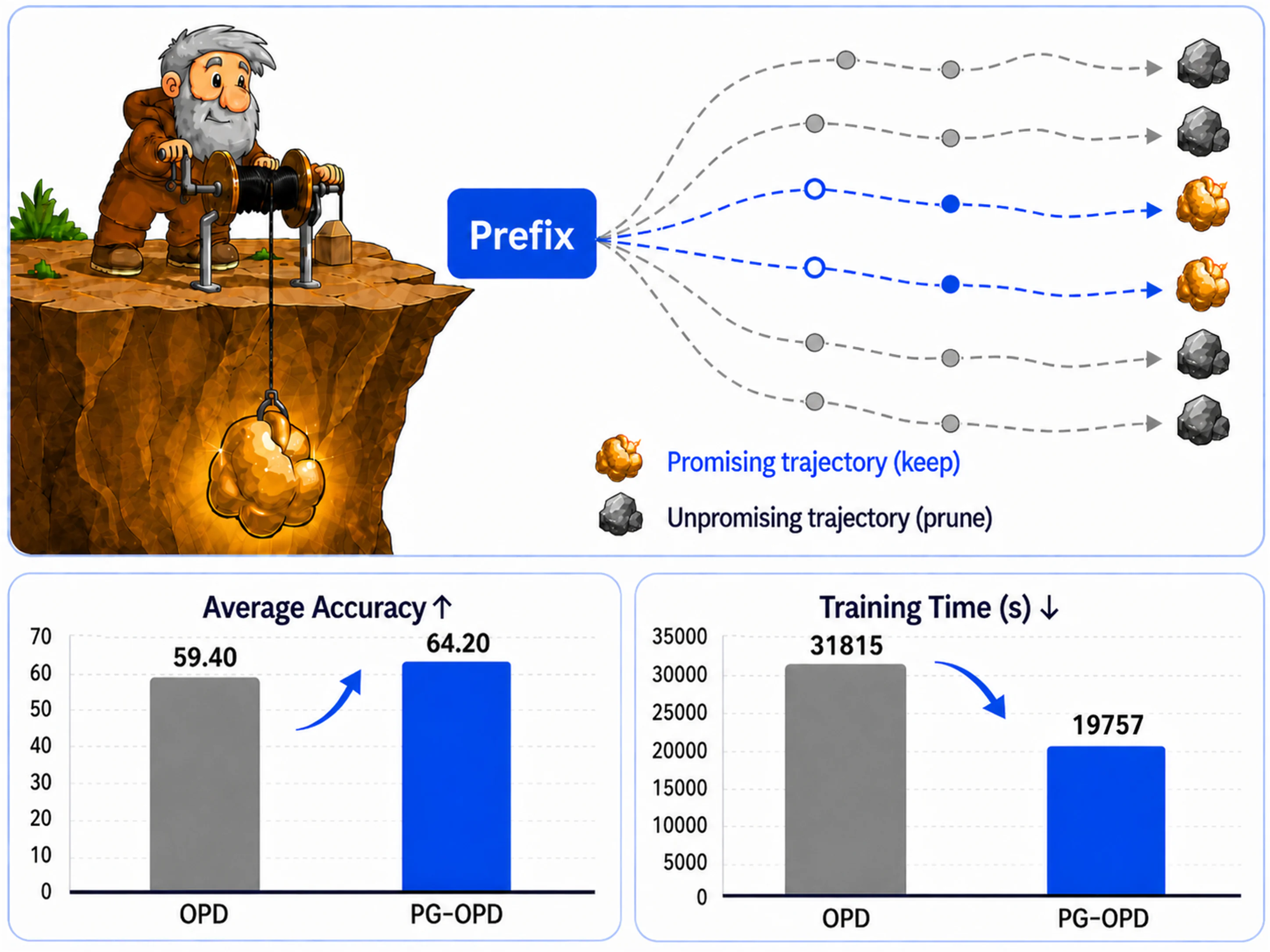
Figure 1: Overview of PG-OPD. Prefix-guided selection identifies high-value trajectories from early prefixes and allocates long-rollout budget to them, improving both avg@16 accuracy and training efficiency. Source: https://arxiv.org/html/2606.21994v2/first_fig_final_2x.png; license: unknown.Figure 1: Overview of PG-OPD. Prefix-guided selection identifies high-value trajectories from early prefixes and allocates long-rollout budget to them, improving both avg@16 accuracy and training efficiency. Source: https://arxiv.org/html/2606.21994v2/first_fig_final_2x.png; license: unknown.
Figure 1 : Overview of SEAD. First, the competence-gated curriculum (left, yellow) selects prompts within the student’s current ability frontier ( d i ≤ c ( t ) d_{i}\leq c(t) ), ensuring rollouts are coherent enough for meaningful supervision. The student π θ \pi_{\theta} generates a rollout, which the teacher π te \pi_{\text{te}} scores with per-token logits. From these, we compute joint entropy ( H θ H_{\theta} , H te H_{\text{te}} ) and partition tokens into three zones: Zone A (gray)—both models confident, zero gradient ( ∼ 50 % {\sim}50\% of tokens); Zone B (blue)—teacher confident but student uncertain, supervised via reverse KL to sharpen toward the teacher’s mode; Zone C (red)—teacher uncertain at reasoning forks, supervised via forward KL to preserve multi-path diversity. A temporal annealing schedule (bottom-right) modulates Zone C as α ⋅ ℒ FKL + ( 1 − α ) ⋅ ℒ RKL \alpha\cdot\mathcal{L}_{\text{FKL}}+(1-\alpha)\cdot\mathcal{L}_{\text{RKL}} , smoothly transitioning from exploration ( α = 0.8 \alpha{=}0.8 ) to refinement ( α = 0 \alpha{=}0 ) over training. The combined loss updates the student. See Algorithm 1 for the full procedure. Source: https://arxiv.org/html/2606.28562v1/fig/sys_v3.png; license: https://arxiv.org/html/2606.28562#A2.T4.Figure 1 : Overview of SEAD. First, the competence-gated curriculum (left, yellow) selects prompts within the student’s current ability frontier ( d i ≤ c ( t ) d_{i}\leq c(t) ), ensuring rollouts are coherent enough for meaningful supervision. The student π θ \pi_{\theta} generates a rollout, which the teacher π te \pi_{\text{te}} scores with per-token logits. From these, we compute joint entropy ( H θ H_{\theta} , H te H_{\text{te}} ) and partition tokens into three zones: Zone A (gray)—both models confident, zero gradient ( ∼ 50 % {\sim}50\% of tokens); Zone B (blue)—teacher confident but student uncertain, supervised via reverse KL to sharpen toward the teacher’s mode; Zone C (red)—teacher uncertain at reasoning forks, supervised via forward KL to preserve multi-path diversity. A temporal annealing schedule (bottom-right) modulates Zone C as α ⋅ ℒ FKL + ( 1 − α ) ⋅ ℒ RKL \alpha\cdot\mathcal{L}_{\text{FKL}}+(1-\alpha)\cdot\mathcal{L}_{\text{RKL}} , smoothly transitioning from exploration ( α = 0.8 \alpha{=}0.8 ) to refinement ( α = 0 \alpha{=}0 ) over training. The combined loss updates the student. See Algorithm 1 for the full procedure. Source: https://arxiv.org/html/2606.28562v1/fig/sys_v3.png; license: https://arxiv.org/html/2606.28562#A2.T4.
Figure 2 : Overview of UI-MOPD training pipeline. In Stage 1, platform-specific desktop and mobile teachers are obtained by supervised fine-tuning on Uni-GUI trajectories collected from a unified cross-platform harness. In Stage 2, a shared student policy is trained with multi-teacher on-policy distillation, where platform-conditioned routing selects the corresponding teacher to provide reverse-KL guidance together with rule-based rollout rewards. Source: https://arxiv.org/html/2607.04425v2/method.png; license: unknown.Figure 2 : Overview of UI-MOPD training pipeline. In Stage 1, platform-specific desktop and mobile teachers are obtained by supervised fine-tuning on Uni-GUI trajectories collected from a unified cross-platform harness. In Stage 2, a shared student policy is trained with multi-teacher on-policy distillation, where platform-conditioned routing selects the corresponding teacher to provide reverse-KL guidance together with rule-based rollout rewards. Source: https://arxiv.org/html/2607.04425v2/method.png; license: unknown.
Figure 2: Framework of PCSD. The student collects on-policy trajectories via multi-turn interaction, while a frozen, skill-augmented teacher scores the student-generated tokens. PCSD aggregates teacher–student log-probability gaps across multiple time scales with exponential decay, adaptively weights them by local variability, and applies trend modulation and continuous gating to derive token-level distillation weights, which are jointly optimized with the trajectory-reward-based GRPO objective. Source: https://arxiv.org/html/2608.01837v1/method-final.png; license: unknown.Figure 2: Framework of PCSD. The student collects on-policy trajectories via multi-turn interaction, while a frozen, skill-augmented teacher scores the student-generated tokens. PCSD aggregates teacher–student log-probability gaps across multiple time scales with exponential decay, adaptively weights them by local variability, and applies trend modulation and continuous gating to derive token-level distillation weights, which are jointly optimized with the trajectory-reward-based GRPO objective. Source: https://arxiv.org/html/2608.01837v1/method-final.png; license: unknown.
Figure 2: Overview of the RP-OPSD pipeline. RP-OPSD constructs on-policy target-language rollouts, compares solution-conditioned and ablated teacher views to compute the RPT gate, and applies the gate to route distillation toward reasoning-sensitive tokens while anchoring surface-realization tokens to the reference distribution. Source: https://arxiv.org/html/2608.06347v1/pipeline.png; license: unknown.Figure 2: Overview of the RP-OPSD pipeline. RP-OPSD constructs on-policy target-language rollouts, compares solution-conditioned and ablated teacher views to compute the RPT gate, and applies the gate to route distillation toward reasoning-sensitive tokens while anchoring surface-realization tokens to the reference distribution. Source: https://arxiv.org/html/2608.06347v1/pipeline.png; license: unknown.
Figure 2: Overview of MemOPD. Here, a call is a model invocation. (1) MemOPD reconstructs each call, separates sampled actions from later context occurrences, and packs the aligned computations under a shared task prefix. (2) RCE compares packed and independent full vocabulary logits within numerical tolerance. (3) The aligned batch supports PPO over the sampled action domain and full vocabulary teacher guidance over the teacher supervision mask. Source: https://arxiv.org/html/2608.07068v1/memopd_main_method_figure.png; license: unknown.Figure 2: Overview of MemOPD. Here, a call is a model invocation. (1) MemOPD reconstructs each call, separates sampled actions from later context occurrences, and packs the aligned computations under a shared task prefix. (2) RCE compares packed and independent full vocabulary logits within numerical tolerance. (3) The aligned batch supports PPO over the sampled action domain and full vocabulary teacher guidance over the teacher supervision mask. Source: https://arxiv.org/html/2608.07068v1/memopd_main_method_figure.png; license: unknown.
Figure 2: Overview of SkillCDG. The offline stage converts long SKILL business policies into a two-layer constraint dependency graph. The online stage performs SKILL-level retrieval, constraint-level retrieval, dependency closure, and LLM-based compliance judgment. Source: https://arxiv.org/html/2608.08146v1/overview.png; license: unknown.Figure 2: Overview of SkillCDG. The offline stage converts long SKILL business policies into a two-layer constraint dependency graph. The online stage performs SKILL-level retrieval, constraint-level retrieval, dependency closure, and LLM-based compliance judgment. Source: https://arxiv.org/html/2608.08146v1/overview.png; license: unknown.
Figure 2: Overview of SkillLens. Source-specific adapters convert public traces and annotations into Visual Skill Cards (VSCs); multi-step sources yield hierarchical cards, while static sources yield execution-level cards. At inference, SkillLens retrieves candidate VSCs, expands the needed evidence views, conditions a frozen VLM executor on the live screen and selected evidence, and exposes verification cues for observable progress or completion. Source: https://arxiv.org/html/2608.10775v1/skilllens_fig2_system_overview_cropped_v3.png; license: unknown.Figure 2: Overview of SkillLens. Source-specific adapters convert public traces and annotations into Visual Skill Cards (VSCs); multi-step sources yield hierarchical cards, while static sources yield execution-level cards. At inference, SkillLens retrieves candidate VSCs, expands the needed evidence views, conditions a frozen VLM executor on the live screen and selected evidence, and exposes verification cues for observable progress or completion. Source: https://arxiv.org/html/2608.10775v1/skilllens_fig2_system_overview_cropped_v3.png; license: unknown.
Figure 2: Test-Time Self-Evolving Framework consists of four core stages: Exploration, Evaluation, Reflection, and Internalization. During test-time adaptation, π G \pi_{\text{G}} explores the environment to predict coordinates. The Reflector π R \pi_{\text{R}} then assesses the prediction to generate a binary score S S and a step-by-step reasoning R R . The reflection knowledge is internalized via Reflection-Guided On-Policy Self-Distillation to update the grounding policy. To optimize memory efficiency, both π G \pi_{\text{G}} and π R \pi_{\text{R}} share a base model and we alternate between the roles of π G \pi_{\text{G}} and π R \pi_{\text{R}} by switching the active LoRA adapters. Source: https://arxiv.org/html/2608.11191v1/framework.png; license: unknown.Figure 2: Test-Time Self-Evolving Framework consists of four core stages: Exploration, Evaluation, Reflection, and Internalization. During test-time adaptation, π G \pi_{\text{G}} explores the environment to predict coordinates. The Reflector π R \pi_{\text{R}} then assesses the prediction to generate a binary score S S and a step-by-step reasoning R R . The reflection knowledge is internalized via Reflection-Guided On-Policy Self-Distillation to update the grounding policy. To optimize memory efficiency, both π G \pi_{\text{G}} and π R \pi_{\text{R}} share a base model and we alternate between the roles of π G \pi_{\text{G}} and π R \pi_{\text{R}} by switching the active LoRA adapters. Source: https://arxiv.org/html/2608.11191v1/framework.png; license: unknown.
Figure 2: Overview of ICSD. A privileged branch evaluates the student’s on-policy action tokens, while the RL objective provides token-level objective influence. ICSD calibrates this influence and uses it to redistribute the inherited trust allocation before the actor update. Source: https://arxiv.org/html/2608.14945v1/Figures/fig_icsd_method_overview.png; license: unknown.Figure 2: Overview of ICSD. A privileged branch evaluates the student’s on-policy action tokens, while the RL objective provides token-level objective influence. ICSD calibrates this influence and uses it to redistribute the inherited trust allocation before the actor update. Source: https://arxiv.org/html/2608.14945v1/Figures/fig_icsd_method_overview.png; license: unknown.
Figure 2 : VOLD training pipeline: VOLD is a two-stage process to instill reasoning capabilities into a student VLM using a text-only teacher. (Stage 1) , the student’s policy is aligned with the teacher’s via SFT on a corpus of teacher-generated reasoning traces. (Stage 2) , the student is trained with a unified on-policy objective that leverages the same rollouts to compute both a sparse reward for RL(GRPO) and a dense distillation loss against the teacher. This combined signal enhances reasoning without requiring any vision-based reasoning data. At Inference, the resulting student model can effectively reason over novel image-text prompts. Source: https://arxiv.org/html/2510.23497v3/teaser_figure_VOLD.png; license: unknown.Figure 2 : VOLD training pipeline: VOLD is a two-stage process to instill reasoning capabilities into a student VLM using a text-only teacher. (Stage 1) , the student’s policy is aligned with the teacher’s via SFT on a corpus of teacher-generated reasoning traces. (Stage 2) , the student is trained with a unified on-policy objective that leverages the same rollouts to compute both a sparse reward for RL(GRPO) and a dense distillation loss against the teacher. This combined signal enhances reasoning without requiring any vision-based reasoning data. At Inference, the resulting student model can effectively reason over novel image-text prompts. Source: https://arxiv.org/html/2510.23497v3/teaser_figure_VOLD.png; license: unknown.
Figure 1: The overall framework of CORD . Given semantically equivalent audio and text inputs, CORD performs on-policy cross-modal self-distillation within a single model. Audio-conditioned trajectories are aligned to text-conditioned behaviors at two levels: (i) a token-level objective that applies importance-aware and position-aware reverse KL weighting along audio rollouts, and (ii) a sequence-level objective that uses a judge-based reward optimized via GRPO to enforce global reasoning consistency. Source: https://arxiv.org/html/2601.16547v1/framework.png; license: unknown.Figure 1: The overall framework of CORD . Given semantically equivalent audio and text inputs, CORD performs on-policy cross-modal self-distillation within a single model. Audio-conditioned trajectories are aligned to text-conditioned behaviors at two levels: (i) a token-level objective that applies importance-aware and position-aware reverse KL weighting along audio rollouts, and (ii) a sequence-level objective that uses a judge-based reward optimized via GRPO to enforce global reasoning consistency. Source: https://arxiv.org/html/2601.16547v1/framework.png; license: unknown.
Figure 1: Overview of the PRISM pipeline. (a) SFT introduces distributional drift between the policy and the supervision distribution. (b) The alignment stage uses an MoE discriminator with dedicated perception and reasoning experts to repair this drift via adversarial on-policy distillation. (c) The resulting distribution-aligned policy provides a stronger initialization for downstream RLVR. Source: https://arxiv.org/html/2604.28123v3/overview.png; license: unknown.Figure 1: Overview of the PRISM pipeline. (a) SFT introduces distributional drift between the policy and the supervision distribution. (b) The alignment stage uses an MoE discriminator with dedicated perception and reasoning experts to repair this drift via adversarial on-policy distillation. (c) The resulting distribution-aligned policy provides a stronger initialization for downstream RLVR. Source: https://arxiv.org/html/2604.28123v3/overview.png; license: unknown.
Figure 6 : Training Dynamics Analysis of Pure Distillation and GRPO Settings. (a) Average accuracy evolution during on-policy distillation for Qwen3-VL-2B and 4B students. VGS achieves higher accuracy throughout training compared to the standard monolithic baseline. (b) Analysis of the GRPO framework (using Qwen3-VL-2B). Left: VGS combined with GRPO yields the highest accuracy trajectory, outperforming both pure GRPO and GRPO + Standard Distillation. Right: While pure GRPO suffers from length explosion, both distillation methods regularize generation length to match the teacher’s average; however, VGS achieves significantly higher accuracy within this efficient length constraint. Source: https://arxiv.org/html/2606.00564v1/figures/training_curve_all2.png; license: unknown.Figure 6 : Training Dynamics Analysis of Pure Distillation and GRPO Settings. (a) Average accuracy evolution during on-policy distillation for Qwen3-VL-2B and 4B students. VGS achieves higher accuracy throughout training compared to the standard monolithic baseline. (b) Analysis of the GRPO framework (using Qwen3-VL-2B). Left: VGS combined with GRPO yields the highest accuracy trajectory, outperforming both pure GRPO and GRPO + Standard Distillation. Right: While pure GRPO suffers from length explosion, both distillation methods regularize generation length to match the teacher’s average; however, VGS achieves significantly higher accuracy within this efficient length constraint. Source: https://arxiv.org/html/2606.00564v1/figures/training_curve_all2.png; license: unknown.
Figure 8 : Qualitative comparison of teacher-side privileged hints under the same student-facing query. Reasoning hints directly expose the key theorem or solving idea, whereas the visual cue hints used in our framework describe only the question-relevant visual structure grounded in the image. Source: https://arxiv.org/html/2606.05718v1/imgs/case1.png; license: unknown.Figure 8 : Qualitative comparison of teacher-side privileged hints under the same student-facing query. Reasoning hints directly expose the key theorem or solving idea, whereas the visual cue hints used in our framework describe only the question-relevant visual structure grounded in the image. Source: https://arxiv.org/html/2606.05718v1/imgs/case1.png; license: unknown.
Figure 4: Overview of Med-OPD. Med-OPD first constructs an evidence-degraded view of the medical image and an answer-aware teacher prompt. The student generates on-policy rollouts from the original image-question pair, while the teacher evaluates these rollouts under both full-evidence and degraded-evidence conditions to estimate MEA. The resulting MEA signal is used to reallocate distillation strength across rollouts and tokens, encouraging the model to focus on evidence-reliant samples and diagnosis-critical visual tokens. Source: https://arxiv.org/html/2607.16303v1/arch.png; license: unknown.Figure 4: Overview of Med-OPD. Med-OPD first constructs an evidence-degraded view of the medical image and an answer-aware teacher prompt. The student generates on-policy rollouts from the original image-question pair, while the teacher evaluates these rollouts under both full-evidence and degraded-evidence conditions to estimate MEA. The resulting MEA signal is used to reallocate distillation strength across rollouts and tokens, encouraging the model to focus on evidence-reliant samples and diagnosis-critical visual tokens. Source: https://arxiv.org/html/2607.16303v1/arch.png; license: unknown.
Figure 6: Illustrative agreement-on-failure trace. A wrong response from the Qwen3 discovery run has final answer 16 16 while the gold answer is 14 14 ; 93.7 % 93.7\% of its 2,666 response tokens are low-divergence at τ = 0.15 \tau=0.15 . The top panel plots pointwise d t d_{t} , clipped at 1.0 for readability; red markers indicate tokens above the threshold. The bottom strip marks low-divergence tokens in orange and high-divergence tokens in red. Source: https://arxiv.org/html/2607.23731v1/fig_case_agreement_trap_digits.png; license: unknown.Figure 6: Illustrative agreement-on-failure trace. A wrong response from the Qwen3 discovery run has final answer 16 16 while the gold answer is 14 14 ; 93.7 % 93.7\% of its 2,666 response tokens are low-divergence at τ = 0.15 \tau=0.15 . The top panel plots pointwise d t d_{t} , clipped at 1.0 for readability; red markers indicate tokens above the threshold. The bottom strip marks low-divergence tokens in orange and high-divergence tokens in red. Source: https://arxiv.org/html/2607.23731v1/fig_case_agreement_trap_digits.png; license: unknown.
Figure 2: Overview of the ROPD pipeline: two frozen teachers—the aligned original (refusal prior) and the fine-tuned model (task skill)—supply source-routed top- K K KL distillation to a single realigned student. Source: https://arxiv.org/html/2607.27081v1/OPD4realign-pipeline.png; license: unknown.Figure 2: Overview of the ROPD pipeline: two frozen teachers—the aligned original (refusal prior) and the fine-tuned model (task skill)—supply source-routed top- K K KL distillation to a single realigned student. Source: https://arxiv.org/html/2607.27081v1/OPD4realign-pipeline.png; license: unknown.
Figure 2 : Overview of VAD. (a) On-policy counterfactual views. Given the same student-generated prefix, the full-image student produces its next-token distribution, while a fixed teacher evaluates evidence-present and evidence-removed views under the unchanged textual context. (b) Correction attribution. The teacher-view contrast defines an intervention-derived proxy u t u_{t} for the visual evidence direction; projecting the complete teacher correction r t r_{t} onto this proxy yields the attributed component r t vis r_{t}^{\mathrm{vis}} and the proxy-unexplained residual r t res r_{t}^{\mathrm{res}} . (c) Target reconstruction. VAD refines r t vis r_{t}^{\mathrm{vis}} into a budgeted signed shift that supports or refutes candidate tokens and adds it to the student-centered logits to construct q T , t VAD q_{T,t}^{\mathrm{VAD}} . The auxiliary teacher views are used only during training. Source: https://arxiv.org/html/2607.28590v1/overview_v11.png; license: unknown.Figure 2 : Overview of VAD. (a) On-policy counterfactual views. Given the same student-generated prefix, the full-image student produces its next-token distribution, while a fixed teacher evaluates evidence-present and evidence-removed views under the unchanged textual context. (b) Correction attribution. The teacher-view contrast defines an intervention-derived proxy u t u_{t} for the visual evidence direction; projecting the complete teacher correction r t r_{t} onto this proxy yields the attributed component r t vis r_{t}^{\mathrm{vis}} and the proxy-unexplained residual r t res r_{t}^{\mathrm{res}} . (c) Target reconstruction. VAD refines r t vis r_{t}^{\mathrm{vis}} into a budgeted signed shift that supports or refutes candidate tokens and adds it to the student-centered logits to construct q T , t VAD q_{T,t}^{\mathrm{VAD}} . The auxiliary teacher views are used only during training. Source: https://arxiv.org/html/2607.28590v1/overview_v11.png; license: unknown.
Figure 2: Overview of FP-OPD. The student generates an on-policy trajectory, after which the student and teacher distributions are evaluated on the same student-visited prefixes. Continuous visual perturbations produce local output-response directions whose span approximates the student-supported visual response space. FP-OPD projects the centered teacher–student gap onto this space under the Fisher metric, constructs the reachable target q R q^{R} , and optimizes it with full-vocabulary reverse KL. Source: https://arxiv.org/html/2608.01263v2/Figures/method.png; license: unknown.Figure 2: Overview of FP-OPD. The student generates an on-policy trajectory, after which the student and teacher distributions are evaluated on the same student-visited prefixes. Continuous visual perturbations produce local output-response directions whose span approximates the student-supported visual response space. FP-OPD projects the centered teacher–student gap onto this space under the Fisher metric, constructs the reachable target q R q^{R} , and optimizes it with full-vocabulary reverse KL. Source: https://arxiv.org/html/2608.01263v2/Figures/method.png; license: unknown.
Figure 1: Overview of stable on-policy knowledge distillation. Top (Forward KL): Standard Forward KL triggers explosive gradients when students are ignorant of teacher-preferred tokens (low P S P_{S} ). Veto reformulates the logit-space target to suppress harmful updates to stabilize early optimization. Bottom (Reverse KL) : Standard Reverse KL causes mode collapse and diversity loss. By tuning β \beta , Veto balances generation decisiveness with distributional diversity, allowing the student to capture multiple teacher modes effectively. Source: https://arxiv.org/html/2601.07155v3/figure_overview_wide_v3.png; license: unknown.Figure 1: Overview of stable on-policy knowledge distillation. Top (Forward KL): Standard Forward KL triggers explosive gradients when students are ignorant of teacher-preferred tokens (low P S P_{S} ). Veto reformulates the logit-space target to suppress harmful updates to stabilize early optimization. Bottom (Reverse KL) : Standard Reverse KL causes mode collapse and diversity loss. By tuning β \beta , Veto balances generation decisiveness with distributional diversity, allowing the student to capture multiple teacher modes effectively. Source: https://arxiv.org/html/2601.07155v3/figure_overview_wide_v3.png; license: unknown.
Figure 1 : Illustration of SPoT . Left: An Oracle surgically corrects reasoning errors, yielding positive samples proximal to the model’s original distribution. Top-Right: Unlike DPO’s relative ranking, we leverage an explicit classification loss that proves more effective for reasoning tasks. Bottom-Right: The tethering effect inherent in our reward definition substantially mitigates catastrophic forgetting. Source: https://arxiv.org/html/2603.01683v2/illustration.png; license: unknown.Figure 1 : Illustration of SPoT . Left: An Oracle surgically corrects reasoning errors, yielding positive samples proximal to the model’s original distribution. Top-Right: Unlike DPO’s relative ranking, we leverage an explicit classification loss that proves more effective for reasoning tasks. Bottom-Right: The tethering effect inherent in our reward definition substantially mitigates catastrophic forgetting. Source: https://arxiv.org/html/2603.01683v2/illustration.png; license: unknown.
Figure 2: Teacher versus student token probabilities at the first sampled-token OPD iteration; the sampled-token signal is skewed toward penalizing the current token. Source: arXiv 2603.25562v2; arXiv non-exclusive distribution license.Figure 2: Teacher versus student token probabilities at the first sampled-token OPD iteration; the sampled-token signal is skewed toward penalizing the current token. Source: arXiv 2603.25562v2; arXiv non-exclusive distribution license.
Figure 2: (a) Standard OPD applies uniform supervision to all samples. (b) Our SCOPE framework refines the learning process by first dividing trajectories into correct Ω C \Omega_{C} and incorrect Ω W \Omega_{W} sets, applying dual-path perplexity-based weighting, and finally optimizing the weighted branches via a unified objective. Source: https://arxiv.org/html/2604.10688v2/main_framework_SCOPE_v3.png; license: unknown.Figure 2: (a) Standard OPD applies uniform supervision to all samples. (b) Our SCOPE framework refines the learning process by first dividing trajectories into correct Ω C \Omega_{C} and incorrect Ω W \Omega_{W} sets, applying dual-path perplexity-based weighting, and finally optimizing the weighted branches via a unified objective. Source: https://arxiv.org/html/2604.10688v2/main_framework_SCOPE_v3.png; license: unknown.
Figure 2: Overview of the Uni-OPD framework. ( Left ) Offline difficulty-aware and online correctness-aware data balancing promote student exploration. ( Right ) Outcome-guided margin calibration mechanism improves the reliability of teacher supervision. ( Middle ) The resulting student policy merges complementary capabilities from multiple domain-specific teachers more effectively than standard OPD, leading to stronger overall performance. Source: https://arxiv.org/html/2605.03677v2/framework.png; license: unknown.Figure 2: Overview of the Uni-OPD framework. ( Left ) Offline difficulty-aware and online correctness-aware data balancing promote student exploration. ( Right ) Outcome-guided margin calibration mechanism improves the reliability of teacher supervision. ( Middle ) The resulting student policy merges complementary capabilities from multiple domain-specific teachers more effectively than standard OPD, leading to stronger overall performance. Source: https://arxiv.org/html/2605.03677v2/framework.png; license: unknown.
Figure 2: The ROPD Pipeline. A Rubricator induces prompt-specific rubrics by contrasting teacher and student rollouts, which a Verifier then utilizes to provide rewards for on-policy optimization. Source: https://arxiv.org/html/2605.07396v1/figures/framework.png; license: unknown.Figure 2: The ROPD Pipeline. A Rubricator induces prompt-specific rubrics by contrasting teacher and student rollouts, which a Verifier then utilizes to provide rewards for on-policy optimization. Source: https://arxiv.org/html/2605.07396v1/figures/framework.png; license: unknown.
Figure 2 : Overview of BRTS. The left panel shows teacher and student trajectories in the trajectory space. The upper-right panel illustrates the selection rule: choose a correct teacher rollout when available, select the student-nearest one when multiple correct rollouts exist, and inject the ground-truth answer when all sampled rollouts are wrong. The lower panels describe the loss computation, where token matching is performed under noisy student context and clean teacher context, respectively. Source: https://arxiv.org/html/2605.09725v3/pipeline-neurips-2026.png; license: unknown.Figure 2 : Overview of BRTS. The left panel shows teacher and student trajectories in the trajectory space. The upper-right panel illustrates the selection rule: choose a correct teacher rollout when available, select the student-nearest one when multiple correct rollouts exist, and inject the ground-truth answer when all sampled rollouts are wrong. The lower panels describe the loss computation, where token matching is performed under noisy student context and clean teacher context, respectively. Source: https://arxiv.org/html/2605.09725v3/pipeline-neurips-2026.png; license: unknown.
Figure 1 : Overview. We map the OP(S)D design space (left, top) and its task-dependent success/failure behavior (left, bottom), identify three failure mechanisms—prefix-distorted teacher state, biased Top- K K reverse-KL, and PI-marginalized OPSD policy (middle), and propose practical fixes: stable Top- K K losses, SFT stabilization, and RLVR-adapted teachers (right). Source: https://arxiv.org/html/2605.11182v2/overview.png; license: unknown.Figure 1 : Overview. We map the OP(S)D design space (left, top) and its task-dependent success/failure behavior (left, bottom), identify three failure mechanisms—prefix-distorted teacher state, biased Top- K K reverse-KL, and PI-marginalized OPSD policy (middle), and propose practical fixes: stable Top- K K losses, SFT stabilization, and RLVR-adapted teachers (right). Source: https://arxiv.org/html/2605.11182v2/overview.png; license: unknown.
Figure 1: Illustration of the foresight mechanism in OPD. Compared with RL, OPD identifies critical modules and aligns with the final optimization direction early in training, concentrating effective updates while reducing redundancy. Based on this, we propose EffOPD, which extrapolates along the early predicted direction to accelerate training. Source: https://arxiv.org/html/2605.11739v3/introfig.png; license: unknown.Figure 1: Illustration of the foresight mechanism in OPD. Compared with RL, OPD identifies critical modules and aligns with the final optimization direction early in training, concentrating effective updates while reducing redundancy. Based on this, we propose EffOPD, which extrapolates along the early predicted direction to accelerate training. Source: https://arxiv.org/html/2605.11739v3/introfig.png; license: unknown.
Figure 1: Illustration of our post-training recipe for building a long-context reasoning model. Source: https://arxiv.org/html/2605.12227v2/images/Intro.png; license: unknown.Figure 1: Illustration of our post-training recipe for building a long-context reasoning model. Source: https://arxiv.org/html/2605.12227v2/images/Intro.png; license: unknown.
Figure 1: RWOPD training and evaluation pipeline. A curriculum-SFT-seeded 7B+LoRA student samples K K rollouts; the open SymbiYosys+Z3 PEC keeps and reward-weights EQUIVALENT or one-sided-implication outputs; the frozen CodeV-SVA-14B teacher then supplies a dense forward-KL target on the kept tokens, with gradients flowing only into the LoRA adapter. The same PEC also defines a sparse RLVF reward used as a controlled baseline; final pass@ k k is reported via JasperGold. Source: https://arxiv.org/html/2605.13501v1/overview.png; license: unknown.Figure 1: RWOPD training and evaluation pipeline. A curriculum-SFT-seeded 7B+LoRA student samples K K rollouts; the open SymbiYosys+Z3 PEC keeps and reward-weights EQUIVALENT or one-sided-implication outputs; the frozen CodeV-SVA-14B teacher then supplies a dense forward-KL target on the kept tokens, with gradients flowing only into the LoRA adapter. The same PEC also defines a sparse RLVF reward used as a controlled baseline; final pass@ k k is reported via JasperGold. Source: https://arxiv.org/html/2605.13501v1/overview.png; license: unknown.
Figure 3: Workflow of ADWIN. The top row performs synchronous OPD updates on the current prefix window L t L_{t} : student rollouts are truncated at the shared window, teacher feedback is evaluated on the prefix, and the resulting loss is used for training updates. The middle probe path asynchronously continues a small probe batch of unfinished prefixes into delayed full-rollout probes. Returned probes are then used in the bottom audit panel to compute prefix–full gradient cosine for candidate window lengths, after which the scheduler updates L t + 1 L_{t+1} by choosing the shortest length whose alignment exceeds the admissibility threshold ρ ∗ \rho^{\ast} . Source: https://arxiv.org/html/2605.28396v1/overview_v3.png; license: unknown.Figure 3: Workflow of ADWIN. The top row performs synchronous OPD updates on the current prefix window L t L_{t} : student rollouts are truncated at the shared window, teacher feedback is evaluated on the prefix, and the resulting loss is used for training updates. The middle probe path asynchronously continues a small probe batch of unfinished prefixes into delayed full-rollout probes. Returned probes are then used in the bottom audit panel to compute prefix–full gradient cosine for candidate window lengths, after which the scheduler updates L t + 1 L_{t+1} by choosing the shortest length whose alignment exceeds the admissibility threshold ρ ∗ \rho^{\ast} . Source: https://arxiv.org/html/2605.28396v1/overview_v3.png; license: unknown.
Figure 5 : Overview of COPSD. The framework first performs a Cross-SFT cold-start to obtain a constitution-conditioned teacher, and then applies constitution-conditioned on-policy distillation, where the teacher provides token-level supervision on the student’s rollouts. Source: https://arxiv.org/html/2606.03089v3/4_methodpipe.png; license: unknown.Figure 5 : Overview of COPSD. The framework first performs a Cross-SFT cold-start to obtain a constitution-conditioned teacher, and then applies constitution-conditioned on-policy distillation, where the teacher provides token-level supervision on the student’s rollouts. Source: https://arxiv.org/html/2606.03089v3/4_methodpipe.png; license: unknown.
Figure 12 : Cosine similarity between student and teacher representations in the shared ℝ r \mathbb{R}^{r} subspace, before and after Stage 1 bridge training, as a function of rank r r . Before training (gray dashed), the two models’ projected representations are essentially orthogonal at all ranks. After training (blue solid), similarity peaks at r = 8 r\!=\!8 ( 95.0 % 95.0\% ) and then decreases monotonically as r r increases, reaching 77.0 % 77.0\% at r = 2048 r\!=\!2048 (full rank). The sweet spot at low rank validates the low-pass filter intuition: the top principal components capture the well-aligned “low-frequency” structure, while higher-rank components introduce architecture-specific noise that degrades alignment. Source: https://arxiv.org/html/2606.06021v4/Figure/rank_cosine.png; license: unknown.Figure 12 : Cosine similarity between student and teacher representations in the shared ℝ r \mathbb{R}^{r} subspace, before and after Stage 1 bridge training, as a function of rank r r . Before training (gray dashed), the two models’ projected representations are essentially orthogonal at all ranks. After training (blue solid), similarity peaks at r = 8 r\!=\!8 ( 95.0 % 95.0\% ) and then decreases monotonically as r r increases, reaching 77.0 % 77.0\% at r = 2048 r\!=\!2048 (full rank). The sweet spot at low rank validates the low-pass filter intuition: the top principal components capture the well-aligned “low-frequency” structure, while higher-rank components introduce architecture-specific noise that degrades alignment. Source: https://arxiv.org/html/2606.06021v4/Figure/rank_cosine.png; license: unknown.
核心问题 / 背景
LM-head 概率监督会受 tokenizer、词表尾部与输出校准限制,跨架构教师尤其困难。
具体方法
在学生 on-policy 状态上对齐中间表示,并用投影/层匹配处理深度与宽度差异,把监督从 output distribution 移到 latent space。
实验设置和结果
数学、科学与代码 reasoning 上比较 output-level OPD;表示对齐提高信息带宽,但要求白盒 hidden states 和额外对齐模块。
Figure 1: Overview of RG-OPD . The student samples trajectories and receives verifier rewards A i A_{i} . The reward–teacher gate keeps a trajectory ( g i = 1 g_{i}{=}1 ) only when the teacher–student likelihood gap is directionally consistent with the reward: L T > L S L_{T}>L_{S} for correct trajectories and L T < L S L_{T}<L_{S} for incorrect ones. The reverse-KL distillation loss is computed exclusively over kept trajectories. Source: https://arxiv.org/html/2607.04037v1/figures/digram3.png; license: unknown.Figure 1: Overview of RG-OPD . The student samples trajectories and receives verifier rewards A i A_{i} . The reward–teacher gate keeps a trajectory ( g i = 1 g_{i}{=}1 ) only when the teacher–student likelihood gap is directionally consistent with the reward: L T > L S L_{T}>L_{S} for correct trajectories and L T < L S L_{T}<L_{S} for incorrect ones. The reverse-KL distillation loss is computed exclusively over kept trajectories. Source: https://arxiv.org/html/2607.04037v1/figures/digram3.png; license: unknown.
Figure 1: Architecture of EasyOPD . The user layer provides configuration-based invocation, the EasyOPD layer encapsulates method-local OPD logic, and verl provides distributed execution. Hooks for loss, rollout, reward, alignment, and teacher-side computation connect method modules to verl, allowing supported methods to share the same execution backend and be selected via YAML configurations. Source: https://arxiv.org/html/2607.11012v1/framework_0526.png; license: unknown.Figure 1: Architecture of EasyOPD . The user layer provides configuration-based invocation, the EasyOPD layer encapsulates method-local OPD logic, and verl provides distributed execution. Hooks for loss, rollout, reward, alignment, and teacher-side computation connect method modules to verl, allowing supported methods to share the same execution backend and be selected via YAML configurations. Source: https://arxiv.org/html/2607.11012v1/framework_0526.png; license: unknown.
Figure 1: Comparison of post-training pipelines. (a) Direct Optimization : The target model is optimized directly using reward feedback. (b) Policy Exploration and Alignment : Policies are independently optimized into experts and then used to align the target model through distribution matching. (c) Asynchronous Proxy Exploration and Update Transfer (Ours) : Proxy policies are explored independently, with their relative on-policy updates extracted and transferred to the target model. Source: https://arxiv.org/html/2607.11505v2/pipeline_v3.png; license: unknown.Figure 1: Comparison of post-training pipelines. (a) Direct Optimization : The target model is optimized directly using reward feedback. (b) Policy Exploration and Alignment : Policies are independently optimized into experts and then used to align the target model through distribution matching. (c) Asynchronous Proxy Exploration and Update Transfer (Ours) : Proxy policies are explored independently, with their relative on-policy updates extracted and transferred to the target model. Source: https://arxiv.org/html/2607.11505v2/pipeline_v3.png; license: unknown.
Figure 3: Pass@k of Qwen3-1.7B-Base trained with OPD variants; gains at low k converge at high k. Source: arXiv 2607.13399v1; CC BY 4.0.Figure 3: Pass@k of Qwen3-1.7B-Base trained with OPD variants; gains at low k converge at high k. Source: arXiv 2607.13399v1; CC BY 4.0.
Figure 4: Case study on MathVerse. Compared with the Base model, our method produces a shorter and more effective reasoning process, reduces redundant intermediate steps, and correctly identifies the key geometric relationships required for solving the problem. Source: https://arxiv.org/html/2607.19046v1/figmaincase.png; license: unknown.Figure 4: Case study on MathVerse. Compared with the Base model, our method produces a shorter and more effective reasoning process, reduces redundant intermediate steps, and correctly identifies the key geometric relationships required for solving the problem. Source: https://arxiv.org/html/2607.19046v1/figmaincase.png; license: unknown.
Figure 2 : Overview of OPOD . Student rollouts are routed by input modality to the corresponding teacher trained offline with GRPO. OPOD combines one-sided token guidance, modality-specific constraint control, and teacher-based verification through answer confidence and reasoning gain. The resulting policy loss, teacher constraint, and reference regularizer jointly update the shared student. Source: https://arxiv.org/html/2607.20918v3/method.png; license: unknown.Figure 2 : Overview of OPOD . Student rollouts are routed by input modality to the corresponding teacher trained offline with GRPO. OPOD combines one-sided token guidance, modality-specific constraint control, and teacher-based verification through answer confidence and reasoning gain. The resulting policy loss, teacher constraint, and reference regularizer jointly update the shared student. Source: https://arxiv.org/html/2607.20918v3/method.png; license: unknown.
Figure 3: Overview of Relay-OPD. Unlike standard OPD (top), which trains on student-only trajectories that continue misdirected after prefix failure, Relay-OPD constructs relay trajectories (middle): when the handoff trigger (bottom) detects that the teacher would redirect the reasoning while the student would not, the teacher briefly takes over before the student resumes. The entire rollout runs in a single speculative decoding engine (right; § 3.3 ). Source: https://arxiv.org/html/2607.26057v1/method.png; license: unknown.Figure 3: Overview of Relay-OPD. Unlike standard OPD (top), which trains on student-only trajectories that continue misdirected after prefix failure, Relay-OPD constructs relay trajectories (middle): when the handoff trigger (bottom) detects that the teacher would redirect the reasoning while the student would not, the teacher briefly takes over before the student resumes. The entire rollout runs in a single speculative decoding engine (right; § 3.3 ). Source: https://arxiv.org/html/2607.26057v1/method.png; license: unknown.
Fig. 5: Overview of Value-aware On-Policy Distillation (VaOPD). Left : The student samples multiple on-policy reasoning trajectories under the standard authenticity query. Middle : An EMA self-teacher, additionally conditioned on training-only labels and perceptual guidance, scores the same student-generated token prefixes and provides dense privileged supervision without generating separate responses. Right : VaOPD models the varying value of these signals at three levels: trajectory weighting prioritizes incorrect rollouts, token weighting emphasizes positions with larger teacher–student discrepancies, and adaptive direction strengthens knowledge transfer at corrective tokens. Source: https://arxiv.org/html/2607.27113v1/vaopd.png; license: unknown.Fig. 5: Overview of Value-aware On-Policy Distillation (VaOPD). Left : The student samples multiple on-policy reasoning trajectories under the standard authenticity query. Middle : An EMA self-teacher, additionally conditioned on training-only labels and perceptual guidance, scores the same student-generated token prefixes and provides dense privileged supervision without generating separate responses. Right : VaOPD models the varying value of these signals at three levels: trajectory weighting prioritizes incorrect rollouts, token weighting emphasizes positions with larger teacher–student discrepancies, and adaptive direction strengthens knowledge transfer at corrective tokens. Source: https://arxiv.org/html/2607.27113v1/vaopd.png; license: unknown.
Figure 3 : Overview of Flux-OPD. (a) illustrates the iterative training process, which divides a single training run into K K iterations, each consisting of context extraction and context distillation. (b) illustrates the contextual correction strategy, which corrects the distillation target by combining the context-free teacher distribution with contextual difference signals from context-conditioned teachers. (c) illustrates the contextual weighting strategy, which further adjusts correction strengths using the conflict term as an indicator, strengthening corrections when context-conditioned teacher distributions are consistent and weakening them when they conflict. Source: https://arxiv.org/html/2607.28022v1/method.png; license: unknown.Figure 3 : Overview of Flux-OPD. (a) illustrates the iterative training process, which divides a single training run into K K iterations, each consisting of context extraction and context distillation. (b) illustrates the contextual correction strategy, which corrects the distillation target by combining the context-free teacher distribution with contextual difference signals from context-conditioned teachers. (c) illustrates the contextual weighting strategy, which further adjusts correction strengths using the conflict term as an indicator, strengthening corrections when context-conditioned teacher distributions are consistent and weakening them when they conflict. Source: https://arxiv.org/html/2607.28022v1/method.png; license: unknown.
Figure 2 : Pipeline of DASH-OPD’s switching mechanism. DASH-OPD accumulates teacher-student discrepancy into drift and recovery evidence, enabling adaptive and bidirectional switching between these two models. Source: https://arxiv.org/html/2607.29078v2/figs/fig2.png; license: unknown.Figure 2 : Pipeline of DASH-OPD’s switching mechanism. DASH-OPD accumulates teacher-student discrepancy into drift and recovery evidence, enabling adaptive and bidirectional switching between these two models. Source: https://arxiv.org/html/2607.29078v2/figs/fig2.png; license: unknown.
Figure 2: Overview of the proposed SA-OPD framework. Given an on-policy rollout, SA-OPD computes teacher–student divergence under the original prompt and a residual no-prompt context. If the divergence barely changes after prompt removal, the teacher signal is likely dominated by input-agnostic priors. SA-OPD filters tokens that are both weakly input-grounded and high-impact, enabling OPD to update from input-grounded distillation signals rather than spurious signals. Source: https://arxiv.org/html/2608.03632v1/2.png; license: unknown.Figure 2: Overview of the proposed SA-OPD framework. Given an on-policy rollout, SA-OPD computes teacher–student divergence under the original prompt and a residual no-prompt context. If the divergence barely changes after prompt removal, the teacher signal is likely dominated by input-agnostic priors. SA-OPD filters tokens that are both weakly input-grounded and high-impact, enabling OPD to update from input-grounded distillation signals rather than spurious signals. Source: https://arxiv.org/html/2608.03632v1/2.png; license: unknown.
Figure 1: Pass@K across AMC2023 and AIME2024/2025/2026; OPD leads at small K while base catches up or surpasses it at large K. Source: arXiv 2608.11829v2; arXiv non-exclusive distribution license.Figure 1: Pass@K across AMC2023 and AIME2024/2025/2026; OPD leads at small K while base catches up or surpasses it at large K. Source: arXiv 2608.11829v2; arXiv non-exclusive distribution license.
Figure 2: Overview of CROP. Validated original-paraphrase-counterfactual triplets enable matched rescoring of a fixed student rollout. CROP ranks tokens by counterfactual minus paraphrase sensitivity and applies a batch-global binary mask to sampled-token OPD. Source: https://arxiv.org/html/2608.13387v2/method.png; license: unknown.Figure 2: Overview of CROP. Validated original-paraphrase-counterfactual triplets enable matched rescoring of a fixed student rollout. CROP ranks tokens by counterfactual minus paraphrase sensitivity and applies a batch-global binary mask to sampled-token OPD. Source: https://arxiv.org/html/2608.13387v2/method.png; license: unknown.
Figure 1: Overview of Step-Level On-Policy Distillation (SOPD). The left and center panels compare On-Policy Distillation (OPD), On-Policy Expert Correction (OEC), and SOPD. The right panel illustrates the packed attention mask used for efficient training. We pack the input prompt, the complete student trajectory, and its multiple step-level teacher targets into a single sequence, enabling these step-level supervision instances to be processed in parallel within a single forward pass to ensure training efficiency. Each teacher target can attend only to the input prompt, its corresponding student prefix, and its own preceding causal teacher tokens, while future student steps and other teacher targets remain masked. Source: https://arxiv.org/html/2608.16333v1/sopd_method_overview_v7.png; license: unknown.Figure 1: Overview of Step-Level On-Policy Distillation (SOPD). The left and center panels compare On-Policy Distillation (OPD), On-Policy Expert Correction (OEC), and SOPD. The right panel illustrates the packed attention mask used for efficient training. We pack the input prompt, the complete student trajectory, and its multiple step-level teacher targets into a single sequence, enabling these step-level supervision instances to be processed in parallel within a single forward pass to ensure training efficiency. Each teacher target can attend only to the input prompt, its corresponding student prefix, and its own preceding causal teacher tokens, while future student steps and other teacher targets remain masked. Source: https://arxiv.org/html/2608.16333v1/sopd_method_overview_v7.png; license: unknown.
Figure 2: Overview of GC-OPD. GC-OPD computes group-normalized verifier rewards and trajectory-level OPD scores, forms their signed residual, and uses RACA to distribute the residual across response tokens while retaining the original OPD advantage. Source: https://arxiv.org/html/2608.19181v1/gcopd_method_overview.png; license: unknown.Figure 2: Overview of GC-OPD. GC-OPD computes group-normalized verifier rewards and trajectory-level OPD scores, forms their signed residual, and uses RACA to distribute the residual across response tokens while retaining the original OPD advantage. Source: https://arxiv.org/html/2608.19181v1/gcopd_method_overview.png; license: unknown.
Figure 3: Overview of the proposed Reasoning-Progress-Aware Reward Filtering OPD. Adjacent reasoning spans with consistent progress signals are first merged. For each merged segment, we sum its process rewards and average its token-level KL divergences. Rank conflicts between the resulting segment-level signals are then used to identify unreliable spans, which are masked during the OPD policy update. Source: https://arxiv.org/html/2608.19408v1/Figures/reasoning_progress_aware_reward_filtering_for_OPD.png; license: unknown.Figure 3: Overview of the proposed Reasoning-Progress-Aware Reward Filtering OPD. Adjacent reasoning spans with consistent progress signals are first merged. For each merged segment, we sum its process rewards and average its token-level KL divergences. Rank conflicts between the resulting segment-level signals are then used to identify unreliable spans, which are masked during the OPD policy update. Source: https://arxiv.org/html/2608.19408v1/Figures/reasoning_progress_aware_reward_filtering_for_OPD.png; license: unknown.
Figure 4: Overview of SpikeOPD. On the same detached self-generated prefixes, teacher correction transfers the ANN distribution, policy anchoring constrains departure from the frozen reference SNN, and spike regularization controls selected-layer firing rates. Only θ \theta is updated. Source: https://arxiv.org/html/2608.27857v1/overview.png; license: unknown.Figure 4: Overview of SpikeOPD. On the same detached self-generated prefixes, teacher correction transfers the ANN distribution, policy anchoring constrains departure from the frozen reference SNN, and spike regularization controls selected-layer firing rates. Only θ \theta is updated. Source: https://arxiv.org/html/2608.27857v1/overview.png; license: unknown.